


 Abstract
 HTML
HTML Reference
 Related
 PDF
PDF


-
The medium
$ NN $ cross sections in transport mode simulations play a crucial role in intermediate-energy heavy ion collisions (HIC), as they significantly influence the predictions of reaction dynamics, collective flow, stopping power, and particle productions [1−9]. In the transport model simulations, the in-medium$ NN\to N\Delta $ cross sections are a critical component of the$ \pi-N-\Delta $ loops, which can effect the pion multiplicity data. The$ \pi^-/\pi^+ $ ratio serves as a sensitive observable for probing the symmetry energy at suprasaturation density. For reproducing the pion multiplicity data, the in-medium$ NN\rightarrow N\Delta $ cross section ($ \sigma^*_{NN\rightarrow N\Delta} $ ) is one of the important ingredients because it will directly influence the first ∆ production which can decay into nucleon and pion or rescatter with nucleons.Many transport codes adopted the free space
$ NN\rightarrow N\Delta $ cross section, i.e., the$ \sigma_{NN\rightarrow N\Delta}^{\text{free}} $ taken from Ref. [10], or phenomenological in-medium cross section, i.e.,$ \sigma_{NN\rightarrow N\Delta}^{*}=R \sigma_{NN\rightarrow N\Delta}^{\text{free}} $ , in the collision integral of transport models [11]. Recent transport model comparison studies by the transport model evaluation project (TMEP) collaboration highlight the large model dependence in pion yields and the need for improved in-medium inputs [12−18]. The isospin independent microscopic approaches have been employed to investigate the in-medium$ NN\rightarrow N\Delta $ cross sections in symmetric nuclear matter [19−25], where the medium correction factorRis the same for for all channels of the$ NN\rightarrow N\Delta $ process. For the isospin asymmetric nuclear matter, Li el at. studied the in-medium$ NN\to N\Delta $ cross section without considering the mass distribution of ∆ resonance and threshold effects by using the relativistic Boltzmann-Uehling-Uhlenbeck (RBUU) microscopic transport theory based on the closed time-path Green's function technique in Ref. [26].In our previous work [27], the in-medium
$ NN\rightarrow N\Delta $ cross section$ \sigma^*_{NN\rightarrow N\Delta} $ by considering the threshold effect and the mass distribution of the ∆ resonance in asymmetric nuclear matter. Further, the dependence of medium correction factorRon the relativistic mean field parameters was investigated in our previous work [28]. With 3 RMF models, i.e., NL$ \rho\delta $ [29], DDMEδ[30], DDRH$ \rho\delta $ [31], our results show thatRincreases with the slope parameterLwhen usingδparameter sets for a given isospin asymmetry. To better understand the influence of theδmeson on the in-medium$ NN\to N\Delta $ cross sections, we compared calculations ofRperformed with and withoutδ-meson parameter sets in our subsequent work [32]. The results indicate that, when using parameter sets without theδmeson, the cross-section factors satisfy$ R_{pp \to n\Delta ^{++}} < R_{nn \to p\Delta ^{-}} $ and$ R_{NN \to N\Delta ^{+}} However, with more than 300 available mean field models, there exists large uncertainty in these cross section results. Therefore, it is essential to reduce the in-medium
$ NN\rightarrow N\Delta $ cross sections, especially because they are increasingly vital for improving transport models — particularly in the context of pion production and for further constraining the symmetry energy at suprasaturation densities. In this paper, we provide reductions on the range of values for the in-medium$ NN\rightarrow N\Delta $ cross sections in isospin asymmetric nuclear matter, based on a selected subset of RMF models that have been constrained by neutron star observations, as discussed in our previous work [33].The paper is organized as follows. First, we briefly describe the properties of nuclear matter for different RMF models. Next, we discuss the constraints on the in-medium correction factorRfor
$ NN\rightarrow N\Delta $ cross sections. Finally, we provide a summary of our findings.For the calculation of the in-medium
$ NN\rightarrow N\Delta $ cross section in nuclear matter, we employ a one-boson exchange model based on a relativistic Lagrangian that includes both nucleons and ∆. According to the structure of the Lagrangian, three types of RMF parameter sets are adopted to estimate the in-medium cross section, as discussed in Ref. [34]: (i) nonlinear models, (ii) density-dependent models, and (iii) point-coupling models. Detailed descriptions of these RMF models are provided in Appendix A. Subsequently, the in-medium$ NN\rightarrow N\Delta $ cross sections are calculated based on the respective RMF Lagrangians, and the detailed derivation of the cross sections can be found in Appendix B.We employ the same RMF Lagrangian to derive the nuclear matter properties, as detailed in Appendix A. Here, the binding energy per particle in asymmetric nuclear matter is expressed as follows:
$ E(\rho,\alpha)=\frac{\epsilon}{\rho}-m_{N}=E_0(\rho)+S(\rho)\alpha^2+O(\alpha^4), $
(1) where the
$ E_0(\rho)=E(\rho,\alpha=0) $ is the binding energy in symmetric nuclear matter and$ S(\rho) $ denotes the symmetry energy. Here,$ \rho = \rho_n + \rho_p $ represents the total nuclear matter density,ϵis the energy density,$ m_{N} $ is the nucleon mass, and$ \alpha = (\rho_n -\rho_p)/(\rho_n +\rho_p) $ is the isospin asymmetry. The nuclear symmetry energy$ S(\rho) $ is defined as$ S(\rho)=\frac{1}{2}\frac{\partial^{2}E(\rho,\alpha)}{\partial \alpha^{2}}\mid_{\alpha=0}. $
(2) The symmetry energy is expanded in terms of
$ (\rho-\rho_0)/3\rho_0 $ :$ S(\rho)=J+\frac{L}{3\rho_0}(\rho-\rho_0)+\frac{K_{sym}}{2}\frac{(\rho-\rho_0)^2}{\rho^2_0}+\cdots . $
(3) Here,
$ J=S(\rho_0) $ represents the symmetry energy at saturation density$ \rho_0 $ . The parameters$ L=3\rho_0\frac{\partial S}{\partial \rho}\mid_{\rho=\rho_0} $ and$ K_{sym}=9\rho^2_0\frac{\partial^2 S}{\partial \rho ^2}\mid_{\rho=\rho_0} $ denote the slope and curvature of the symmetry energy at saturation density, respectively.The coupling constants in RMF models are crucial for predicting the in-medium ∆ production cross section as well as for determining the equation of state (EOS) of nuclear matter. To reduce the uncertainty in the in-medium
$ NN\to N\Delta $ cross sections, it is essential to select reasonable RMF models. In previous work [33], the EOS of nuclear matter was constrained using neutron star observations based on various RMF parameter sets. In this study, we calculate the in-medium$ NN\to N\Delta $ cross sections using 180 RMF interaction sets, as described in Refs. [33,35].Furthermore, an important task is to further evaluate the in-medium
$ NN\to N\Delta $ cross sections using the selected RMF parameter sets that have been refined based on multiple neutron star observables from Refs. [33,36,37]. The final constrained RMF models are: HC, FSUGZ03, IU-FSU,$ {\rm{G2}}^{*} $ , BSR8, BSR9, FA3, FZ3, and DD-F. The EOS parameters (incompressibility$ K_0 $ , symmetry energyJ, slope of symmetry energyL, and curvature of symmetry$ K_{sym} $ ) used in this work from with and without NS observations are both listed inTable 1. Additionally, the properties of nuclear matter and related parameters of all RMF models used here are detailed inTable C1of Appendix C.$ K_0 $ (MeV)J(MeV) L(MeV) $ K_{sym} $ (MeV)With neutron star constraint 216.87–297.75 29.70–31.62 29.08–69.86 -275.05–28.99 Without neutron star constraint 199.92–300.67 17.37–43.54 29.08–140.37 -275.05–398.27 Table 1.Ranges of the EOS from the used RMF models.
As a key step in calculating the in-medium cross sections (see Eq. 48 in Appendix B), it is first necessary to determine the Dirac effective masses of nucleons, the effective pole masses of ∆ resonances, and the channel-dependent changes in vector self-energies. These quantities must be obtained based on the RMF parameter sets that have been constrained as described earlier.
In theFig. 1, we plot the effective mass of the nucleon (
$ m^*_{N}/m_{N} $ ) and effective pole masses of ∆ ($ m^*_{0,\Delta}/m_{0,\Delta} $ ) as function of$ \rho/\rho_0 $ in symmetric nuclear matter. Except for NL$ \rho\delta $ A [29], NL$ \rho\delta $ B [29], DDMEδ[30] and DDRH$ \rho\delta $ [31], all others included the constraint RMF models are without-δmodels. Consequently, these models do not exhibit mass splitting between protons and neutrons (or among different ∆ isospin states). Therefore, we only show the effective masses in symmetric nuclear matter.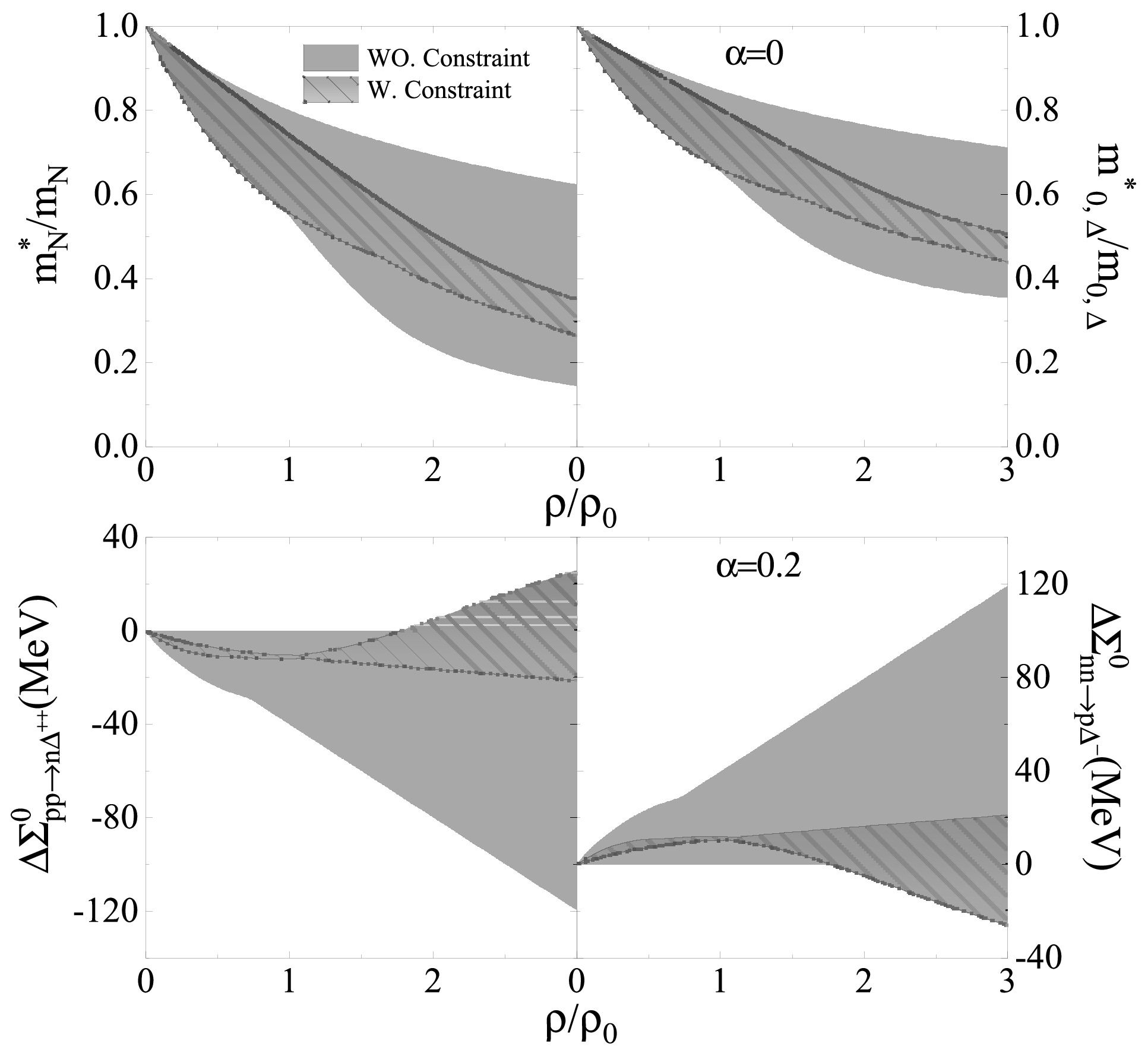
Figure 1.(Color online) The upper panels show the effective mass of the nucleon (
$ m^*_{N}/m_{N} $ ) and effective pole masses of ∆ ($ m^*_{0,\Delta}/m_{0,\Delta} $ ) in symmetric nuclear matter as functions of$ \rho/\rho_0 $ . The lower panels display the changes in vector self-energies$ \Delta \Sigma^{0}{pp \to n\Delta^{++}} $ and$ \Delta \Sigma^{0}{nn \to p\Delta^{-}} $ in asymmetric nuclear matter with$ \alpha = 0.2 $ . The pure gray areas represent the ranges of all considered RMF models, and the hatched areas indicate the subset constrained by neutron star observations. The constrained shaded band denotes the model-ensemble envelope—range from minimal to maximal values across all RMF interactions that pass the neutron-star filters—and is not a statistical confidence interval.Because the most RMF models are adjusted to describe the nuclei and nuclear matter in the density region from near subsaturation density
$ \rho\approx2/3\rho_0 $ (which represents the average value between the central and surface densities [38−43]) up to saturation density, significant uncertainties remain regarding RMF model properties—such as effective masses—at densities above$ \rho_0 $ .From the results inFig. 1, we can see that the uncertainty of the effective masses reduced, i.e., the range of
$ \Delta m^*_{N}=\dfrac{m^*_{N, max}-m^*_{N,min}}{m_{N}}=0.196 $ (corresponding to$ m^*_{N}/m_{N}=0.551-0.747 $ ) at$ \rho_0 $ , while$ m^*_{N}/m_{N}= 0.677- 0.709 $ (corresponding to$ \Delta m^*_{N} $ =0.032) are deduced at 68% confidence level from just three types of momentum dependence of the optical potential model in Ref. [44]. Additionally, the range of$ \Delta m^*_{0,\Delta} $ are also decreased, especially at the density above saturation density.From our previous work [32], we observed that there remains a splitting among different channels of the in-medium
$ NN\to N\Delta $ cross sections in asymmetric nuclear matter. To illustrate this effect, we present the vector self-energy changes for two representative channels in asymmetric matter at$ \alpha = 0.2 $ :$ \Delta \Sigma^{0}_{pp\to n\Delta^{++}}=\Sigma^{0}_p+\Sigma^{0}_p-\Sigma^{0}_n-\Sigma^{0}_{\Delta^{++}}, $
and
$ \Delta \Sigma^{0}_{nn\to p\Delta^-}=\Sigma^{0}_n+\Sigma^{0}_n-\Sigma^{0}_p-\Sigma^{0}_{\Delta^-}. $
These channels,
$ pp \to n\Delta^{++} $ and$ nn \to p\Delta^{-} $ , are highlighted because they are the main contributors to the$ NN \to N\Delta $ processes.The results indicate that the uncertainties in both the effective masses and the vector self-energy changes are significantly reduced when using the constrained RMF models, especially at higher densities. Consequently, the uncertainties in the in-medium
$ NN\to N\Delta $ cross sections are expected to be correspondingly diminished.Fig. 2displays the in-medium
$pp\to n\Delta^{++}$ cross sections as a function of the total energy$\sqrt{s}$ in symmetric nuclear matter. The left panel compares the cross sections in free space and at saturation density, while the middle and right panels present the cross sections$\sigma^*_{pp\to n\Delta^{++}}$ at$\rho=2\rho_0$ and$3\rho_0$ , respectively. Compared with the unconstrained results, the constrained in-medium cross sections show a notably reduced spread, particularly at densities above$\rho_0$ . This reduction in uncertainty of in-medium cross section is consistent with the behaviors of the nucleon and$\Delta$ effective masses shown inFig. 1. The in-medium$ NN \to N\Delta $ cross section depends explicitly on the effective masses ($ m^*_N $ and$ m^*_{0,\Delta} $ ) in symmetric nuclear matter (the channel-dependent vector self-energy changes$ \Delta \Sigma^0 $ should be also considered in asymmetric nuclear matter), which can be derived from Appendix B. Bulk “nuclear-matter properties” such as$ K_0 $ ,J,Land$ K_{sym} $ do not enter the cross-section formula directly, which are determined by RMF interactions. After applying neutron-star constraints, the surviving RMF sets develop similar trajectories of$ m^*(\rho) $ and$ \Delta \Sigma^0(\rho) $ at 2 to 3$ \rho_0 $ , which lead to the observed narrowing of in-medium cross sections, even though the spread in incompressibility of the same sets may remain sizable (e.g. FA3 and FZ3).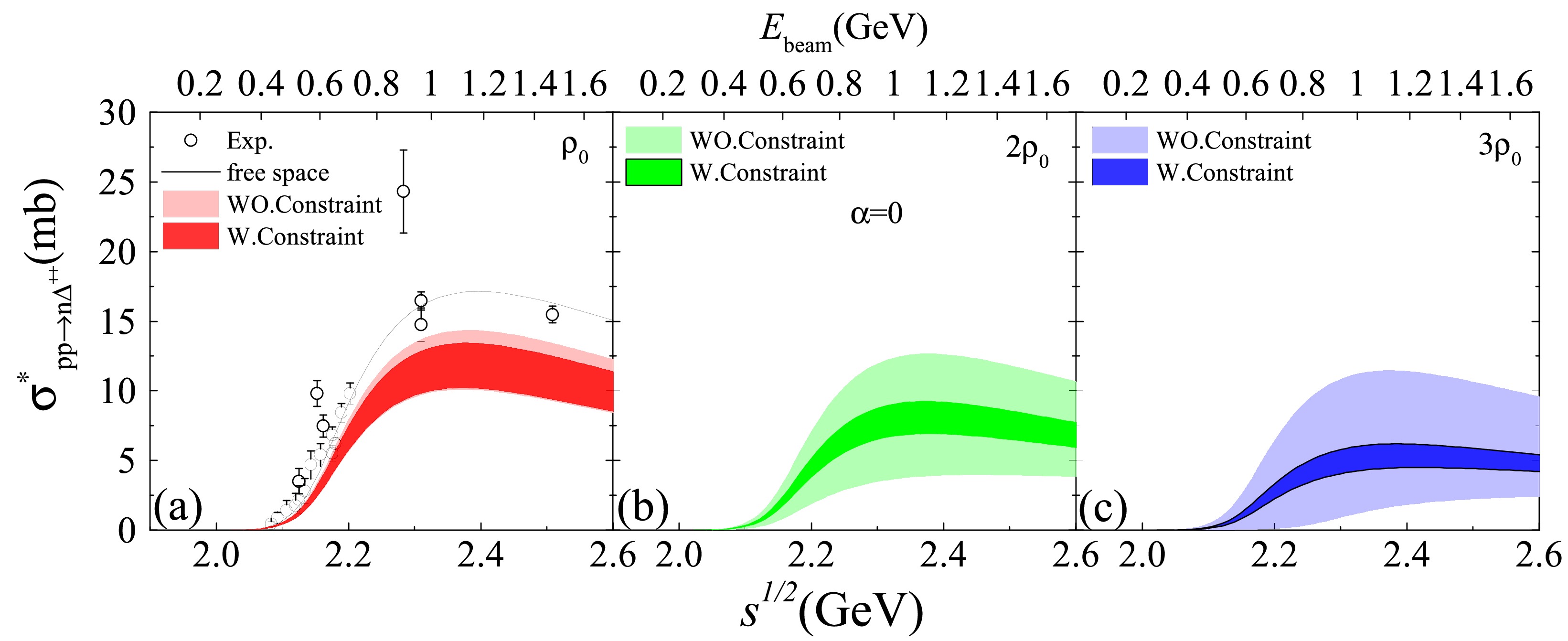
Figure 2.(Color online) The in-medium
$pp \to n\Delta^{++}$ cross section as function of$ \sqrt{s} $ in symmetric nuclear matter. The left panel shows the cross section in free space and at$\rho_0 $ , while the middle and right panels present results at$ 2\rho_0 $ and$ 3\rho_0 $ , respectively. The experimental data are taken from Ref. [45].Since there is no isospin splitting of effective masses in symmetric nuclear matter, the in-medium cross section for
$ nn\rightarrow p\Delta^{-} $ is identical to that for$ pp\rightarrow n\Delta^{++} $ . Cross sections for other channels can be obtained by applying the appropriate isospin Clebsch-Gordan coefficients, yielding values equal to$ \frac{1}{3}\sigma^*_{pp\rightarrow n\Delta^{++}} $ . Consequently, the ratio$ R=\sigma^*_{NN\rightarrow N\Delta}/\sigma_{NN\rightarrow N\Delta} $ is the same for all channels of$ NN\rightarrow N\Delta $ in symmetric nuclear matter.Fig. 3shows the medium correction factorsR(top panels) and the corresponding range
$\Delta R = R_{\max} - R_{\min}$ (bottom panels) as a function of$\rho/\rho_0$ for beam energies$E_{\mathrm{beam}} = 0.4, 0.8,$ and$1.2$ GeV in symmetric nuclear matter. The unconstrained$\Delta R$ increases with density, but once constraints are applied to the in-medium cross sections, the spread inRis notably reduced compared to the unconstrained results. For instance, at$E_{\mathrm{beam}} = 0.4$ GeV,$\Delta R$ decreases from$0.283$ to$0.219$ at$\rho_0$ , from$0.648$ to$0.182$ at$2\rho_0$ , and from$0.696$ to$0.125$ at$3\rho_0$ . This reduction stems from the decreased uncertainty in effective masses (seeFig. 1).
Figure 3.(Color online) The upper panels areRas a function of density
$\rho/\rho_0$ at beam energy$E_{beam}=0.4$ , 0.8, and 1.2 GeV in symmetric nuclear matter. The lower panels display the corresponding range$\Delta R$ .Here we take the
$pp\to n\Delta^{++}$ and$nn\to p \Delta^{-}$ channels as examples to illustrate the in-medium cross sections in asymmetric nuclear matter. InFig. 4, we plotRfor$pp\to n\Delta^{++}$ (panels (a), (b), (c)) and$nn\to p \Delta^{-}$ (panels (d), (e), (f)), the constrained median values$R_{\mathrm{med}}$ (panels (g), (h), (i)), and the range$\Delta R$ (panels (j), (k), (l)) as functions of$\rho/\rho_0$ in asymmetric nuclear matter with$\alpha=0.2$ for$E_{\mathrm{beam}}=0.4$ , 0.8, and 1.2 GeV.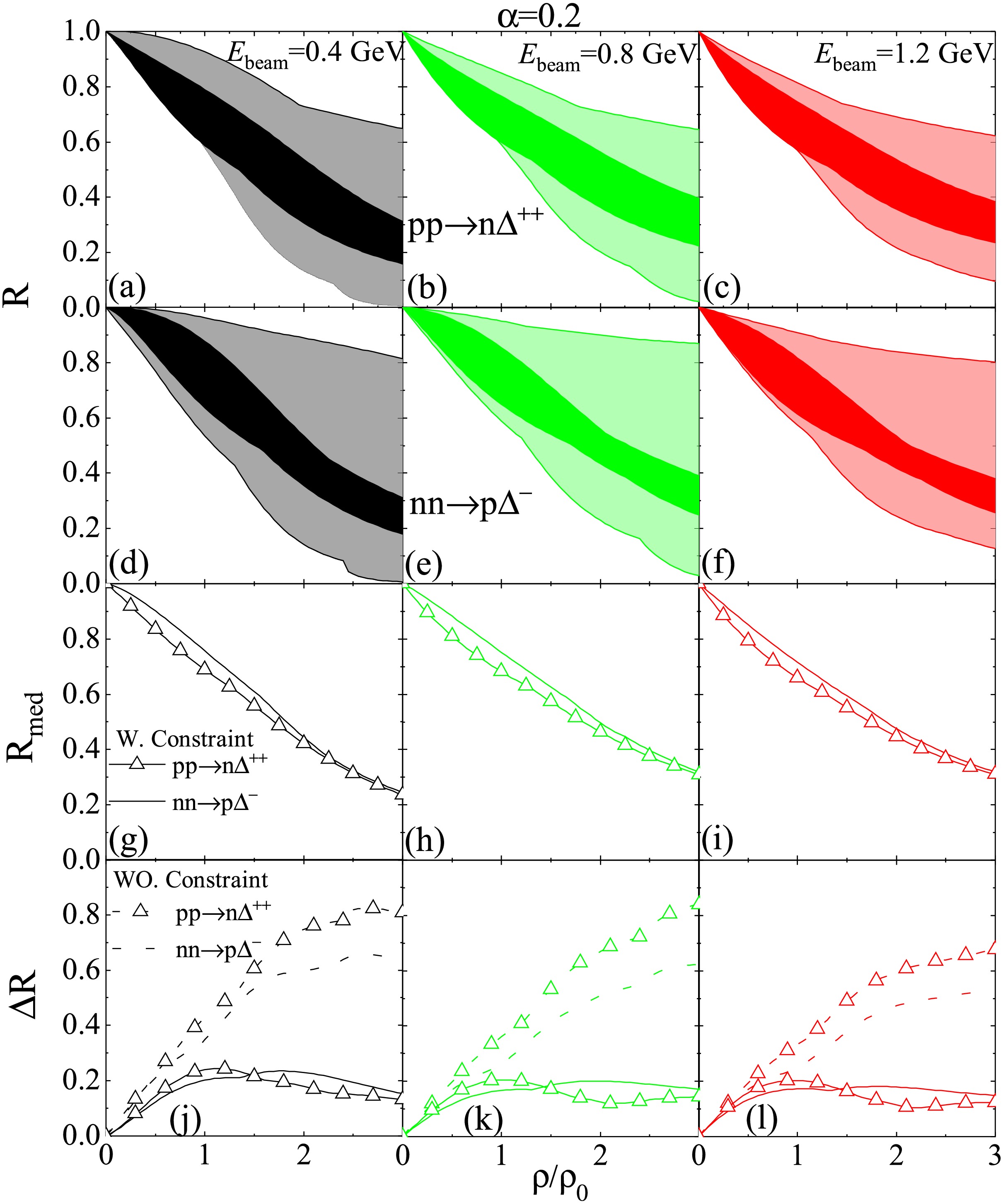
Figure 4.(Color online) The in-medium correction factorRfor
$pp\to n\Delta^{++}$ (a, b, c panels) and$nn\to p \Delta^{-}$ (d,e,f panels), the constraint median values of correction factors$R_{med}$ (g, h, i panels), and$\Delta R$ (j, k, l panels) as function of density$\rho/\rho_0$ in asymmetric nuclear matter with$\alpha=0.2$ .It is also evident that the constrained median values of the in-medium
$NN\to N\Delta$ cross sections follow$ R_{pp\to n\Delta^{++}} < R_{nn\to p \Delta^{-}} $ , consistent with Ref. [32].Furthermore, the constrained correction factorsRin asymmetric nuclear matter are notably smaller than their unconstrained counterparts. For instance, at
$\rho_0$ ,$\Delta R_{pp\to n\Delta^{++}}$ decreases from 0.347 to 0.202, while$\Delta R_{nn\to p\Delta^{-}}$ decreases from 0.427 to 0.238. Similar reductions are observed at$2\rho_0$ and$3\rho_0$ . For example, at$2\rho_0$ ,$\Delta R_{pp\to n\Delta^{++}}$ decreases from 0.593 to 0.230, whereas$\Delta R_{nn\to p\Delta^{-}}$ decreases from 0.746 to 0.178. Overall, the restricted$\Delta R$ decreases by about 42%–44%, 61%–76%, and 76%–84% from$pp\to n\Delta^{++}$ to$nn\to p\Delta^{-}$ at at$ \rho_0 $ ,$ 2\rho_0 $ and$ 3\rho_0 $ respectively for$ E_{beam}=0.4 $ GeV, as well as for other beam energies.Evaluating the in-medium
$NN \to N\Delta$ cross sections in asymmetric nuclear matter is crucial for heavy-ion collision studies, as it provides a potential avenue for reducing uncertainties in the symmetry energy at suprasaturation densities. To facilitate their application in transport models, we present parameterizations of the constrained in-medium cross section correction factorsRfor all$NN \to N\Delta$ channels at beam energies$E_{\mathrm{beam}}=0.4, 0.6, 0.8, 1.0,$ and$1.2$ GeV, both in symmetric and asymmetric nuclear matter.In summary, we present the evaluated the in-medium
$NN\rightarrow N\Delta$ cross sections derived from RMF parameter sets constrained by neutron star observations [33]. Compared to the unconstrained results, our findings show that the ranges of$\sigma^*_{NN\rightarrow N\Delta}$ are significantly reduced over the density range$0 < \rho \leq 3\rho_0$ for beam energies of$E_{\mathrm{beam}} = 0.4,\, 0.8,$ and$1.2$ GeV in both symmetric and asymmetric nuclear matter, especially at densities above$\rho_0$ . For completeness, the parameterized forms of the in-medium$NN\rightarrow N\Delta$ cross-section corrections are given in the supplemental material.We hope the constrained in-medium cross sections will help reduce the uncertainties of information on the symmetry energy at high densities by facilitating them in the prediction of pion observables in QMD models to simulate heavy-ion collision experiments, such as those performed by the HADES (Au+Au) [46] and MSU (Sn+Sn) [15]. However, matter created in heavy ion collisions is hot and in a non-equilibrium state, implying that the in-medium
$ NN\to N\Delta $ cross section depends on temperature. Prior work has explored the temperature dependence of in-medium nucleon-nucleon scattering cross sections (see Ref. [47]), reporting a possible enhancement at finite temperature relative to the cold matter case. The explicit temperature dependence of in-medium$ NN\to N\Delta $ cross sections is rarely discussed, and we will investigate it in future work. -
The medium
$ NN $ cross sections in transport mode simulations play a crucial role in intermediate-energy heavy ion collisions (HIC), as they significantly influence the predictions of reaction dynamics, collective flow, stopping power, and particle productions [1−9]. In the transport model simulations, the in-medium$ NN\to N\Delta $ cross sections are a critical component of the$ \pi-N-\Delta $ loops, which can effect the pion multiplicity data. The$ \pi^-/\pi^+ $ ratio serves as a sensitive observable for probing the symmetry energy at suprasaturation density. For reproducing the pion multiplicity data, the in-medium$ NN\rightarrow N\Delta $ cross section ($ \sigma^*_{NN\rightarrow N\Delta} $ ) is one of the important ingredients because it will directly influence the first ∆ production which can decay into nucleon and pion or rescatter with nucleons.Many transport codes adopted the free space
$ NN\rightarrow N\Delta $ cross section, i.e., the$ \sigma_{NN\rightarrow N\Delta}^{\text{free}} $ taken from Ref. [10], or phenomenological in-medium cross section, i.e.,$ \sigma_{NN\rightarrow N\Delta}^{*}=R \sigma_{NN\rightarrow N\Delta}^{\text{free}} $ , in the collision integral of transport models [11]. Recent transport model comparison studies by the transport model evaluation project (TMEP) collaboration highlight the large model dependence in pion yields and the need for improved in-medium inputs [12−18]. The isospin independent microscopic approaches have been employed to investigate the in-medium$ NN\rightarrow N\Delta $ cross sections in symmetric nuclear matter [19−25], where the medium correction factorRis the same for for all channels of the$ NN\rightarrow N\Delta $ process. For the isospin asymmetric nuclear matter, Li el at. studied the in-medium$ NN\to N\Delta $ cross section without considering the mass distribution of ∆ resonance and threshold effects by using the relativistic Boltzmann-Uehling-Uhlenbeck (RBUU) microscopic transport theory based on the closed time-path Green's function technique in Ref. [26].In our previous work [27], the in-medium
$ NN\rightarrow N\Delta $ cross section$ \sigma^*_{NN\rightarrow N\Delta} $ by considering the threshold effect and the mass distribution of the ∆ resonance in asymmetric nuclear matter. Further, the dependence of medium correction factorRon the relativistic mean field parameters was investigated in our previous work [28]. With 3 RMF models, i.e., NL$ \rho\delta $ [29], DDMEδ[30], DDRH$ \rho\delta $ [31], our results show thatRincreases with the slope parameterLwhen usingδparameter sets for a given isospin asymmetry. To better understand the influence of theδmeson on the in-medium$ NN\to N\Delta $ cross sections, we compared calculations ofRperformed with and withoutδ-meson parameter sets in our subsequent work [32]. The results indicate that, when using parameter sets without theδmeson, the cross-section factors satisfy$ R_{pp \to n\Delta ^{++}} < R_{nn \to p\Delta ^{-}} $ and$ R_{NN \to N\Delta ^{+}} However, with more than 300 available mean field models, there exists large uncertainty in these cross section results. Therefore, it is essential to reduce the in-medium
$ NN\rightarrow N\Delta $ cross sections, especially because they are increasingly vital for improving transport models — particularly in the context of pion production and for further constraining the symmetry energy at suprasaturation densities. In this paper, we provide reductions on the range of values for the in-medium$ NN\rightarrow N\Delta $ cross sections in isospin asymmetric nuclear matter, based on a selected subset of RMF models that have been constrained by neutron star observations, as discussed in our previous work [33].The paper is organized as follows. First, we briefly describe the properties of nuclear matter for different RMF models. Next, we discuss the constraints on the in-medium correction factorRfor
$ NN\rightarrow N\Delta $ cross sections. Finally, we provide a summary of our findings.For the calculation of the in-medium
$ NN\rightarrow N\Delta $ cross section in nuclear matter, we employ a one-boson exchange model based on a relativistic Lagrangian that includes both nucleons and ∆. According to the structure of the Lagrangian, three types of RMF parameter sets are adopted to estimate the in-medium cross section, as discussed in Ref. [34]: (i) nonlinear models, (ii) density-dependent models, and (iii) point-coupling models. Detailed descriptions of these RMF models are provided in Appendix A. Subsequently, the in-medium$ NN\rightarrow N\Delta $ cross sections are calculated based on the respective RMF Lagrangians, and the detailed derivation of the cross sections can be found in Appendix B.We employ the same RMF Lagrangian to derive the nuclear matter properties, as detailed in Appendix A. Here, the binding energy per particle in asymmetric nuclear matter is expressed as follows:
$ E(\rho,\alpha)=\frac{\epsilon}{\rho}-m_{N}=E_0(\rho)+S(\rho)\alpha^2+O(\alpha^4), $
(1) where the
$ E_0(\rho)=E(\rho,\alpha=0) $ is the binding energy in symmetric nuclear matter and$ S(\rho) $ denotes the symmetry energy. Here,$ \rho = \rho_n + \rho_p $ represents the total nuclear matter density,ϵis the energy density,$ m_{N} $ is the nucleon mass, and$ \alpha = (\rho_n -\rho_p)/(\rho_n +\rho_p) $ is the isospin asymmetry. The nuclear symmetry energy$ S(\rho) $ is defined as$ S(\rho)=\frac{1}{2}\frac{\partial^{2}E(\rho,\alpha)}{\partial \alpha^{2}}\mid_{\alpha=0}. $
(2) The symmetry energy is expanded in terms of
$ (\rho-\rho_0)/3\rho_0 $ :$ S(\rho)=J+\frac{L}{3\rho_0}(\rho-\rho_0)+\frac{K_{sym}}{2}\frac{(\rho-\rho_0)^2}{\rho^2_0}+\cdots . $
(3) Here,
$ J=S(\rho_0) $ represents the symmetry energy at saturation density$ \rho_0 $ . The parameters$ L=3\rho_0\frac{\partial S}{\partial \rho}\mid_{\rho=\rho_0} $ and$ K_{sym}=9\rho^2_0\frac{\partial^2 S}{\partial \rho ^2}\mid_{\rho=\rho_0} $ denote the slope and curvature of the symmetry energy at saturation density, respectively.The coupling constants in RMF models are crucial for predicting the in-medium ∆ production cross section as well as for determining the equation of state (EOS) of nuclear matter. To reduce the uncertainty in the in-medium
$ NN\to N\Delta $ cross sections, it is essential to select reasonable RMF models. In previous work [33], the EOS of nuclear matter was constrained using neutron star observations based on various RMF parameter sets. In this study, we calculate the in-medium$ NN\to N\Delta $ cross sections using 180 RMF interaction sets, as described in Refs. [33,35].Furthermore, an important task is to further evaluate the in-medium
$ NN\to N\Delta $ cross sections using the selected RMF parameter sets that have been refined based on multiple neutron star observables from Refs. [33,36,37]. The final constrained RMF models are: HC, FSUGZ03, IU-FSU,$ {\rm{G2}}^{*} $ , BSR8, BSR9, FA3, FZ3, and DD-F. The EOS parameters (incompressibility$ K_0 $ , symmetry energyJ, slope of symmetry energyL, and curvature of symmetry$ K_{sym} $ ) used in this work from with and without NS observations are both listed inTable 1. Additionally, the properties of nuclear matter and related parameters of all RMF models used here are detailed inTable C1of Appendix C.$ K_0 $ (MeV)J(MeV) L(MeV) $ K_{sym} $ (MeV)With neutron star constraint 216.87–297.75 29.70–31.62 29.08–69.86 -275.05–28.99 Without neutron star constraint 199.92–300.67 17.37–43.54 29.08–140.37 -275.05–398.27 Table 1.Ranges of the EOS from the used RMF models.
As a key step in calculating the in-medium cross sections (see Eq. 48 in Appendix B), it is first necessary to determine the Dirac effective masses of nucleons, the effective pole masses of ∆ resonances, and the channel-dependent changes in vector self-energies. These quantities must be obtained based on the RMF parameter sets that have been constrained as described earlier.
In theFig. 1, we plot the effective mass of the nucleon (
$ m^*_{N}/m_{N} $ ) and effective pole masses of ∆ ($ m^*_{0,\Delta}/m_{0,\Delta} $ ) as function of$ \rho/\rho_0 $ in symmetric nuclear matter. Except for NL$ \rho\delta $ A [29], NL$ \rho\delta $ B [29], DDMEδ[30] and DDRH$ \rho\delta $ [31], all others included the constraint RMF models are without-δmodels. Consequently, these models do not exhibit mass splitting between protons and neutrons (or among different ∆ isospin states). Therefore, we only show the effective masses in symmetric nuclear matter.
Figure 1.(Color online) The upper panels show the effective mass of the nucleon (
$ m^*_{N}/m_{N} $ ) and effective pole masses of ∆ ($ m^*_{0,\Delta}/m_{0,\Delta} $ ) in symmetric nuclear matter as functions of$ \rho/\rho_0 $ . The lower panels display the changes in vector self-energies$ \Delta \Sigma^{0}{pp \to n\Delta^{++}} $ and$ \Delta \Sigma^{0}{nn \to p\Delta^{-}} $ in asymmetric nuclear matter with$ \alpha = 0.2 $ . The pure gray areas represent the ranges of all considered RMF models, and the hatched areas indicate the subset constrained by neutron star observations. The constrained shaded band denotes the model-ensemble envelope—range from minimal to maximal values across all RMF interactions that pass the neutron-star filters—and is not a statistical confidence interval.Because the most RMF models are adjusted to describe the nuclei and nuclear matter in the density region from near subsaturation density
$ \rho\approx2/3\rho_0 $ (which represents the average value between the central and surface densities [38−43]) up to saturation density, significant uncertainties remain regarding RMF model properties—such as effective masses—at densities above$ \rho_0 $ .From the results inFig. 1, we can see that the uncertainty of the effective masses reduced, i.e., the range of
$ \Delta m^*_{N}=\dfrac{m^*_{N, max}-m^*_{N,min}}{m_{N}}=0.196 $ (corresponding to$ m^*_{N}/m_{N}=0.551-0.747 $ ) at$ \rho_0 $ , while$ m^*_{N}/m_{N}= 0.677- 0.709 $ (corresponding to$ \Delta m^*_{N} $ =0.032) are deduced at 68% confidence level from just three types of momentum dependence of the optical potential model in Ref. [44]. Additionally, the range of$ \Delta m^*_{0,\Delta} $ are also decreased, especially at the density above saturation density.From our previous work [32], we observed that there remains a splitting among different channels of the in-medium
$ NN\to N\Delta $ cross sections in asymmetric nuclear matter. To illustrate this effect, we present the vector self-energy changes for two representative channels in asymmetric matter at$ \alpha = 0.2 $ :$ \Delta \Sigma^{0}_{pp\to n\Delta^{++}}=\Sigma^{0}_p+\Sigma^{0}_p-\Sigma^{0}_n-\Sigma^{0}_{\Delta^{++}}, $
and
$ \Delta \Sigma^{0}_{nn\to p\Delta^-}=\Sigma^{0}_n+\Sigma^{0}_n-\Sigma^{0}_p-\Sigma^{0}_{\Delta^-}. $
These channels,
$ pp \to n\Delta^{++} $ and$ nn \to p\Delta^{-} $ , are highlighted because they are the main contributors to the$ NN \to N\Delta $ processes.The results indicate that the uncertainties in both the effective masses and the vector self-energy changes are significantly reduced when using the constrained RMF models, especially at higher densities. Consequently, the uncertainties in the in-medium
$ NN\to N\Delta $ cross sections are expected to be correspondingly diminished.Fig. 2displays the in-medium
$pp\to n\Delta^{++}$ cross sections as a function of the total energy$\sqrt{s}$ in symmetric nuclear matter. The left panel compares the cross sections in free space and at saturation density, while the middle and right panels present the cross sections$\sigma^*_{pp\to n\Delta^{++}}$ at$\rho=2\rho_0$ and$3\rho_0$ , respectively. Compared with the unconstrained results, the constrained in-medium cross sections show a notably reduced spread, particularly at densities above$\rho_0$ . This reduction in uncertainty of in-medium cross section is consistent with the behaviors of the nucleon and$\Delta$ effective masses shown inFig. 1. The in-medium$ NN \to N\Delta $ cross section depends explicitly on the effective masses ($ m^*_N $ and$ m^*_{0,\Delta} $ ) in symmetric nuclear matter (the channel-dependent vector self-energy changes$ \Delta \Sigma^0 $ should be also considered in asymmetric nuclear matter), which can be derived from Appendix B. Bulk “nuclear-matter properties” such as$ K_0 $ ,J,Land$ K_{sym} $ do not enter the cross-section formula directly, which are determined by RMF interactions. After applying neutron-star constraints, the surviving RMF sets develop similar trajectories of$ m^*(\rho) $ and$ \Delta \Sigma^0(\rho) $ at 2 to 3$ \rho_0 $ , which lead to the observed narrowing of in-medium cross sections, even though the spread in incompressibility of the same sets may remain sizable (e.g. FA3 and FZ3).
Figure 2.(Color online) The in-medium
$pp \to n\Delta^{++}$ cross section as function of$ \sqrt{s} $ in symmetric nuclear matter. The left panel shows the cross section in free space and at$\rho_0 $ , while the middle and right panels present results at$ 2\rho_0 $ and$ 3\rho_0 $ , respectively. The experimental data are taken from Ref. [45].Since there is no isospin splitting of effective masses in symmetric nuclear matter, the in-medium cross section for
$ nn\rightarrow p\Delta^{-} $ is identical to that for$ pp\rightarrow n\Delta^{++} $ . Cross sections for other channels can be obtained by applying the appropriate isospin Clebsch-Gordan coefficients, yielding values equal to$ \frac{1}{3}\sigma^*_{pp\rightarrow n\Delta^{++}} $ . Consequently, the ratio$ R=\sigma^*_{NN\rightarrow N\Delta}/\sigma_{NN\rightarrow N\Delta} $ is the same for all channels of$ NN\rightarrow N\Delta $ in symmetric nuclear matter.Fig. 3shows the medium correction factorsR(top panels) and the corresponding range
$\Delta R = R_{\max} - R_{\min}$ (bottom panels) as a function of$\rho/\rho_0$ for beam energies$E_{\mathrm{beam}} = 0.4, 0.8,$ and$1.2$ GeV in symmetric nuclear matter. The unconstrained$\Delta R$ increases with density, but once constraints are applied to the in-medium cross sections, the spread inRis notably reduced compared to the unconstrained results. For instance, at$E_{\mathrm{beam}} = 0.4$ GeV,$\Delta R$ decreases from$0.283$ to$0.219$ at$\rho_0$ , from$0.648$ to$0.182$ at$2\rho_0$ , and from$0.696$ to$0.125$ at$3\rho_0$ . This reduction stems from the decreased uncertainty in effective masses (seeFig. 1).
Figure 3.(Color online) The upper panels areRas a function of density
$\rho/\rho_0$ at beam energy$E_{beam}=0.4$ , 0.8, and 1.2 GeV in symmetric nuclear matter. The lower panels display the corresponding range$\Delta R$ .Here we take the
$pp\to n\Delta^{++}$ and$nn\to p \Delta^{-}$ channels as examples to illustrate the in-medium cross sections in asymmetric nuclear matter. InFig. 4, we plotRfor$pp\to n\Delta^{++}$ (panels (a), (b), (c)) and$nn\to p \Delta^{-}$ (panels (d), (e), (f)), the constrained median values$R_{\mathrm{med}}$ (panels (g), (h), (i)), and the range$\Delta R$ (panels (j), (k), (l)) as functions of$\rho/\rho_0$ in asymmetric nuclear matter with$\alpha=0.2$ for$E_{\mathrm{beam}}=0.4$ , 0.8, and 1.2 GeV.
Figure 4.(Color online) The in-medium correction factorRfor
$pp\to n\Delta^{++}$ (a, b, c panels) and$nn\to p \Delta^{-}$ (d,e,f panels), the constraint median values of correction factors$R_{med}$ (g, h, i panels), and$\Delta R$ (j, k, l panels) as function of density$\rho/\rho_0$ in asymmetric nuclear matter with$\alpha=0.2$ .It is also evident that the constrained median values of the in-medium
$NN\to N\Delta$ cross sections follow$ R_{pp\to n\Delta^{++}} < R_{nn\to p \Delta^{-}} $ , consistent with Ref. [32].Furthermore, the constrained correction factorsRin asymmetric nuclear matter are notably smaller than their unconstrained counterparts. For instance, at
$\rho_0$ ,$\Delta R_{pp\to n\Delta^{++}}$ decreases from 0.347 to 0.202, while$\Delta R_{nn\to p\Delta^{-}}$ decreases from 0.427 to 0.238. Similar reductions are observed at$2\rho_0$ and$3\rho_0$ . For example, at$2\rho_0$ ,$\Delta R_{pp\to n\Delta^{++}}$ decreases from 0.593 to 0.230, whereas$\Delta R_{nn\to p\Delta^{-}}$ decreases from 0.746 to 0.178. Overall, the restricted$\Delta R$ decreases by about 42%–44%, 61%–76%, and 76%–84% from$pp\to n\Delta^{++}$ to$nn\to p\Delta^{-}$ at at$ \rho_0 $ ,$ 2\rho_0 $ and$ 3\rho_0 $ respectively for$ E_{beam}=0.4 $ GeV, as well as for other beam energies.Evaluating the in-medium
$NN \to N\Delta$ cross sections in asymmetric nuclear matter is crucial for heavy-ion collision studies, as it provides a potential avenue for reducing uncertainties in the symmetry energy at suprasaturation densities. To facilitate their application in transport models, we present parameterizations of the constrained in-medium cross section correction factorsRfor all$NN \to N\Delta$ channels at beam energies$E_{\mathrm{beam}}=0.4, 0.6, 0.8, 1.0,$ and$1.2$ GeV, both in symmetric and asymmetric nuclear matter.In summary, we present the evaluated the in-medium
$NN\rightarrow N\Delta$ cross sections derived from RMF parameter sets constrained by neutron star observations [33]. Compared to the unconstrained results, our findings show that the ranges of$\sigma^*_{NN\rightarrow N\Delta}$ are significantly reduced over the density range$0 < \rho \leq 3\rho_0$ for beam energies of$E_{\mathrm{beam}} = 0.4,\, 0.8,$ and$1.2$ GeV in both symmetric and asymmetric nuclear matter, especially at densities above$\rho_0$ . For completeness, the parameterized forms of the in-medium$NN\rightarrow N\Delta$ cross-section corrections are given in the supplemental material.We hope the constrained in-medium cross sections will help reduce the uncertainties of information on the symmetry energy at high densities by facilitating them in the prediction of pion observables in QMD models to simulate heavy-ion collision experiments, such as those performed by the HADES (Au+Au) [46] and MSU (Sn+Sn) [15]. However, matter created in heavy ion collisions is hot and in a non-equilibrium state, implying that the in-medium
$ NN\to N\Delta $ cross section depends on temperature. Prior work has explored the temperature dependence of in-medium nucleon-nucleon scattering cross sections (see Ref. [47]), reporting a possible enhancement at finite temperature relative to the cold matter case. The explicit temperature dependence of in-medium$ NN\to N\Delta $ cross sections is rarely discussed, and we will investigate it in future work.
HTML


-
In this paper, we ignore the Fock term in the relativistic mean field, where models are all Hartree RMF model sets.
1. Nonlinear relativistic mean field
The Lagrangians are nonlinear RMF model are:
$ {\cal{L}}_{NL}={\cal{L}}_F+{\cal{L}}_I, $
(A1) where
$ {\cal{L}}_F $ is,$ \begin{aligned}[b] {\cal{L}}_{F}=\;& \bar{\Psi}[i\gamma_{\mu}\partial^{\mu}-m_{N}]\Psi+\bar{\Delta}_{\lambda}[i\gamma_{\mu}\partial^{\mu}-m_{\Delta}]\Delta^{\lambda} \\& +\frac{1}{2}\left(\partial_{\mu}{\boldsymbol{\pi}}\partial^{\mu}{\boldsymbol{\pi}}-m^{2}_{\pi}{\boldsymbol{\pi}}^{2}\right)+\frac{1}{2}\partial_{\mu}\sigma\partial^{\mu}\sigma-\frac{1}{2}m^{2}_{\sigma}\sigma^{2}-U(\sigma)\\& -\frac{1}{4}\omega_{\mu\nu}\omega^{\mu\nu}+\frac{1}{2}m^{2}_{\omega}\omega_{\mu}\omega^{\mu}+\frac{1}{4}\zeta^{4}(\omega_{\mu}\omega^{\mu})^2\\& -\frac{1}{4}{\boldsymbol{\rho}}_{\mu\nu}{\boldsymbol{\rho}}^{\mu\nu}+\frac{1}{2}m^{2}_{\rho}{\boldsymbol{\rho}}_{\mu}{\boldsymbol{\rho}}^{\mu}+\frac{1}{2}\left(\partial_{\mu}{\boldsymbol{\delta}}\partial^{\mu}{\boldsymbol{\delta}}-m^{2}_{\delta}{\boldsymbol{\delta}}^{2}\right)\\& +g_{\sigma}g^2_{\omega}\sigma \omega_{\mu}\omega^{\mu}( \alpha_1+\frac{1}{2}\alpha^{\prime}_{1}g_{\sigma} ) + g_{\sigma}g^2_{\rho}\sigma {\boldsymbol{\rho}}_{\mu}{\boldsymbol{\rho}}^{\mu}( \alpha_2+\frac{1}{2}\alpha^{\prime}_{2}g_{\sigma} ) \\& +\frac{1}{2}\alpha^{\prime}_{3}g^2_{\omega}g^2_{\rho}\omega_{\mu}\omega^{\mu} {\boldsymbol{\rho}}_{\mu}{\boldsymbol{\rho}}^{\mu}\; . \end{aligned} $
(A2) and
$ {\cal{L}}_I $ is interaction part,$ \begin{aligned}[b]{\cal{L}}_I=\;& g_{\sigma NN}\bar{\Psi}\Psi\sigma-g_{\omega NN}\bar{\Psi}\gamma_{\mu}\Psi\omega^{\mu}-g_{\rho NN}\bar{\Psi}\gamma_{\mu}{\boldsymbol{\tau}} \cdot\Psi{\boldsymbol{\rho}}^{\mu}\\& -\frac{f_{\pi NN}}{m_{\pi}}\bar{\Psi}\gamma_{\mu}\gamma_{5}{\boldsymbol{\tau}} \cdot\Psi\partial^{\mu}{\boldsymbol{\pi}}+g_{\delta NN}\bar{\Psi}{\boldsymbol{\tau}} \cdot\Psi{\boldsymbol{\delta}}\\& +g_{\sigma \Delta \Delta}\bar{\Delta}_{\mu}\Delta^{\mu}\sigma-g_{\omega \Delta \Delta}\bar{\Delta}_{\mu}\gamma_{\nu}\Delta^{\mu}\omega^{\nu} \\& -g_{\rho \Delta\Delta}\bar{\Delta}_{\mu}\gamma_{\nu}{\boldsymbol{\rm{T}}} \cdot\Delta^{\mu}{\boldsymbol{\rho}}^{\nu}+\frac{g_{\pi \Delta\Delta}}{m_{\pi}}\bar{\Delta}_{\mu}\gamma_{\nu}\gamma_{5}{\boldsymbol{\rm{T}}} \cdot\Delta^{\mu}\partial^{\nu}{\boldsymbol{\pi}}\\& +g_{\delta \Delta\Delta}\bar{\Delta}_{\mu}{\boldsymbol{\rm{T}}} \cdot\Delta^{\mu}{\boldsymbol{\delta}}+\frac{g_{\pi N\Delta}}{m_{\pi}}\bar{\Delta}_{\mu}{{{\cal{T}}}}\cdot \Psi\partial^{\mu}{\boldsymbol{\pi}}\\& +\frac{ig_{\rho N\Delta}}{m_{\rho}}\bar{\Delta}_{\mu}\gamma_{\nu}\gamma_{5}{{{\cal{T}}}}\cdot \Psi\left(\partial^{\nu}{\boldsymbol{\rho}}^{\mu}-\partial^{\mu}{\boldsymbol{\rho}}^{\nu}\right)+h.c. \end{aligned}$
(A3) In Eq. (A2),
$ \omega_{\mu\nu} $ and$ {\boldsymbol{\rho}}_{\mu\nu} $ are defined as$ \partial_{\mu}\omega_{\nu}-\partial_{\nu}\omega_{\mu} $ and$ \partial_{\mu}{\boldsymbol{\rho}}_{\nu}-\partial_{\nu}{\boldsymbol{\rho}}_{\mu} $ , respectively. The nonlinear potential of theσfield is given by$ U(\sigma)=\frac{1}{3}g_{2}\sigma^{3}+\frac{1}{4}g_{3}\sigma^{4} $ . Here$ {\boldsymbol{\tau}} $ andTare the isospin matrices for the nucleon and ∆ [48,49], while$ {{{\cal{T}}}} $ is the isospin transition matrix between the isospin 1/2 and the 3/2 fields [10].In the uniform rest nuclear matter, the effective momentum can be written as
$ {\bf{p}}_i^*={\bf{p}}_i $ since the spatial components of vector field vanish, i.e.,$ {\bf{\Sigma}}=0 $ . Thus, in the mean field approach, the effective energy is given by:$ p_i^{*0}=p^{0}_{i}-\Sigma^{0}_{i}, $
(A4) The effective masses of nucleon and ∆ read as:
$ m^{*}_{i}=m_{i}+\Sigma^{S}_{i}, $
(A5) Here
$ \Sigma^{0}_{i} $ and$ \Sigma^{S}_{i} $ represent the vector and scalar self-energy respectively for the RMF parameter sets.The vector and scalar potentials in the nonlinear(NL) RMF model are expressed as:
$ \Sigma^0_{i,NL}=g_{\omega }\bar{\omega}^{0}+g_{\rho }t_{3,i}\bar{\rho}^{0}_3 $
(A6) $ \Sigma^S_{i,NL} =-g_{\sigma }\bar{\sigma}- g_{\delta }t_{3,i}\bar{\delta}_3 $
(A7) where
$ t_{3,i} $ represents the third component of the isospin of the nucleon and ∆, with the following values:$ t_{3,n}=-1 $ ,$ t_{3,p}=1 $ ,$ t_{3,\Delta^{++}}=1 $ ,$ t_{3,\Delta^{+}}=\frac{1}{3} $ ,$ t_{3,\Delta^{0}}=-\frac{1}{3} $ ,$ t_{3,\Delta^{-}}=-1 $ . The$ \bar{\omega}^{0} $ ,$ \bar{\rho}^{0}_3 $ ,$ \bar{\sigma} $ and$ \bar{\delta}_3 $ denote the expectation values of the mesons field in the mean-field approximation. In the RMF model, the equations of motion for the mesons are:$ \begin{aligned}[b] m^{2}\bar{\sigma} =\;& g_{\sigma}\rho_{s}-g_2\bar{\sigma}^2-g_3\bar{\sigma}^3+g_{\sigma}g^2_{\omega}(\bar{\omega}^{0})^2(\alpha_1+\alpha^{\prime}_1 g_{\sigma}\bar{\sigma})\\ & +g_{\sigma}g^2_{\rho}(\bar{\rho}_{3}^{0})^2(\alpha_2+\alpha^{\prime}_2 g_{\sigma}\bar{\sigma}) \end{aligned} $
(A8) $\begin{aligned}[b] m^{2}_{\omega}\bar{\omega}^{0} =\;& g_{\omega}\rho-\zeta g_{\omega}^4(\bar{\omega}^{0})^3-g_{\sigma}g^2_{\omega}\bar{\sigma}\bar{\omega}^{0}(2\alpha_1+\alpha^{\prime}_1 g_{\sigma}\bar{\sigma})\\& -\alpha^{\prime}_3 g^2_{\omega}g^2_{\rho}(\bar{\rho}_{3}^{0})^2\bar{\omega}^{0} \end{aligned}$
(A9) $ \begin{aligned}[b] m^{2}_{\rho}\bar{\rho}_{3}^{0} =\;& g_{\rho}\rho_{3}-g_{\sigma}g^2_{\rho}\bar{\sigma}\bar{\rho}_{3}^{0}(2\alpha_2+\alpha^{\prime}_2 g_{\sigma}\bar{\sigma})\\ &-\alpha^{\prime}_3 g^2_{\omega}g^2_{\rho}\bar{\rho}_{3}^{0}(\bar{\omega}^{0})^2 \end{aligned} $
(A10) $ m^{2}_{\delta}\bar{\delta}_{3} = g_{\delta}\rho_{s3} $
(A11) The nucleon densities are (assuming no ∆ density):
$ \rho_s=\langle \bar{\Psi}\Psi \rangle= \rho_{s n}+\rho_{s p} $
(A12) $ \rho=\langle \bar{\Psi}\gamma^0 \Psi \rangle= \rho_{n}+\rho_{p} $
(A13) $ \rho_{s3}=\langle \bar{\Psi}\tau_3 \Psi \rangle= \rho_{s p}-\rho_{s n} $
(A14) $ \rho_3=\langle \bar{\Psi}\gamma^0 \tau_3 \Psi \rangle= \rho_{p}-\rho_{n} $
(A15) With Fermi momenta
$ k_{F,i} $ fori= n or p, the scalar and vector densities are:$ \begin{aligned}[b] \rho_{si} =\;& \frac{C(i)}{(2\pi)^{3}}\int_{k
(A16) $ \rho_{i} = \frac{C(i)}{(2\pi)^{3}}\int_{k
(A17) where the degeneracy factor
$ C(i=n,p)=2 $ , and$ E^*_{F i}=\sqrt{k_{F i}^{2}+m^{2*}_{i}} $ is the Fermi energy of neutrons and protons.The eigenvalues of neutron and proton from the Dirac equation are:
$ e_{n}=g_{\omega}\bar{\omega}^{0}-g_{\rho}\bar{\rho}_{3}^{0}+\sqrt{k^{2*}_{n}+m^{*2}_{n}}, $
(A18) $ e_{p}=g_{\omega}\bar{\omega}^{0}+g_{\rho}\bar{\rho}_{3}^{0}+\sqrt{k^{2*}_{p}+m^{*2}_{p}}. $
(A19) The expression for the energy density and pressure are obtained from the given Lagrangian using energy momentum tensor relation given by,
$ T^{\mu\nu}=\sum\limits_{i}\frac{\partial {\cal{L}}}{\partial (\partial_{\mu} \phi_{i})}\partial^{\nu} \phi_{i}-g^{\mu\nu} {\cal{L}}, $
(A20) where
$ \phi_{i} $ runs over all possible fields. The energy densityϵand pressurePcan be obtain from the energy-momentum tensor:$\begin{aligned}[b] \epsilon_{NL} =\;& \langle T^{00} \rangle = \frac{1}{2}m^{2}_{\sigma}\bar{\sigma}^{2}+\frac{1}{3}g_{2}\bar{\sigma}^{3}+\frac{1}{4}g_{3}\bar{\sigma}^{4} -\frac{1}{2}m^{2}_{\omega}(\bar{\omega}^{0})^{2}\\ & -\frac{\zeta}{4} g_{\omega}^4(\bar{\omega}^{0})^4+g_{\omega}\bar{\omega}^{0}\rho-\frac{1}{2}m^{2}_{\rho}(\bar{\rho}^{0}_{3})^2+g_{\rho}\bar{\rho}^{0}_{3}\rho_{3}\\&+\frac{1}{2}m^{2}_{\delta}\bar{\delta}_{3}^2 -g_{\sigma}g^2_{\omega}\bar{\sigma}(\bar{\omega}^{0})^2(\alpha_1+\frac{1}{2}\alpha^{\prime}_1 g_{\sigma}\bar{\sigma})\\ & -g_{\sigma}g^2_{\rho}\bar{\sigma}(\bar{\rho}_{3}^{0})^2(\alpha_2+\frac{1}{2}\alpha^{\prime}_2 g_{\sigma}\bar{\sigma})-\frac{1}{2}\alpha^{\prime}_3 g^2_{\omega}g^2_{\rho}(\bar{\rho}_{3}^{0})^2(\bar{\omega}^{0})^2\\&+\frac{1}{4}[3E^*_{F n}\rho_{n}+m^{*}_{n}\rho_{s n}]+\frac{1}{4}[3E^*_{F p}\rho_{p}+m^{*}_{p}\rho_{s p}], \end{aligned}$
(A21) and
$ \begin{aligned}[b] P_{NL} =\;& \frac{1}{3}\sum\limits_{i=1}^{3}\langle T^{ii} \rangle= -\frac{1}{2}m^{2}_{\sigma}\bar{\sigma}^{2}-\frac{1}{3}g_{2}\bar{\sigma}^{3}-\frac{1}{4}g_{3}\bar{\sigma}^{4}\\ & +\frac{1}{2}m^{2}_{\omega}(\bar{\omega}^{0})^{2}+\frac{\zeta}{4} g_{\omega}^4(\bar{\omega}^{0})^4+\frac{1}{2}m^{2}_{\rho}(\bar{\rho}^{0}_{3})^2\\ & -\frac{1}{2}m^{2}_{\delta}\bar{\delta}_{3}^2+g_{\sigma}g^2_{\omega}\bar{\sigma}(\bar{\omega}^{0})^2(\alpha_1+\frac{1}{2}\alpha^{\prime}_1 g_{\sigma}\bar{\sigma})\\ & +g_{\sigma}g^2_{\rho}\bar{\sigma}(\bar{\rho}_{3}^{0})^2(\alpha_2+\frac{1}{2}\alpha^{\prime}_2 g_{\sigma}\bar{\sigma})+\frac{1}{2}\alpha^{\prime}_3 g^2_{\omega}g^2_{\rho}(\bar{\rho}_{3}^{0})^2(\bar{\omega}^{0})^2\\ & +\frac{1}{4}[E^*_{F n}\rho_{n}-m^{*}_{n}\rho_{s n}]+\frac{1}{4}[E^*_{F p}\rho_{p}-m^{*}_{p}\rho_{s p}]. \end{aligned} $
(A22) The same calculations for density-dependence and point-coupling models can be found in Refs.[30,31,50−52].
For symmetric nuclear matter,
$ m^{*}_{n}=m^{*}_{p}=m^{*}_{N} $ since$ \bar{\delta}_{3} $ vanishes.The expressions of the symmetry energy and slope of symmetry energy L for nonlinear RMF models are:
$ \begin{aligned}[b] S(\rho)_{NL}=\;& \frac{k_{F}^{2}}{6E^*_{F}}+\frac{1}{2}\rho\frac{g^2_{\rho}}{m^{*2}_{\rho}}\\ &-\frac{1}{2}\rho\left(\frac{\dfrac{g^2_{\delta}}{m^{2}_{\delta}}m^{* 2}_{N}}{E^{*2}_{F}\left[1+\dfrac{g^2_{\delta}}{m^{2}_{\delta}}A(\rho,m^*_{N})\right]}\right), \end{aligned} $
(A23) where
$ m^{*2}_{\rho}=m^{2}_{\rho}+g_{\sigma}g^2_{\rho}\bar{\sigma}(2\alpha_2+\alpha^{\prime}_2 g_{\sigma}\bar{\sigma})+\alpha^{\prime}_3 g^2_{\omega}g^2_{\rho}(\bar{\omega}^{0})^2 $ , and$ A(\rho,m^*_{N})=3\left( \frac{\rho_s}{m^*_{N}} -\frac{\rho}{E^*_{F}} \right) . $
(A24) $ \begin{aligned}[b] L_{NL} =\;& \frac{k^{2}_{F}}{3E^{*}_{F}}\left( 1-\frac{k^{2}_{F}}{2E^{*2}_{F}} -\frac{k^{3}_{F}m^*_{N}}{E^{*2}_{F}\pi^2}\frac{\partial m^*_{N}}{\partial \rho}\right) \\ & +\frac{3g^{2}_{\rho}}{2m^{*2}_\rho}\rho\left( 1-\frac{1}{m^{*2}_{\rho}}\frac{\partial m^{*2}_{\rho}}{\partial \rho}\rho\right) \\ & -\frac{1}{2}\rho\left(\frac{\dfrac{g^2_{\delta}}{m^{2}_{\delta}}m^{* 2}_{N}}{E^{*2}_{F}\left[1+\dfrac{g^2_{\delta}}{m^{2}_{\delta}}A(\rho,m^*_{N})\right]}\right)\\ &\times\Bigg\{3-\frac{2k^{2}_{F}}{E^{*2}_{F}}+6\left(1-\frac{m^{*2}_{N}}{E^{*2}_{F}}\right)\frac{\rho}{m^{*}_{N}}\frac{\partial m^{*}_{N}}{\partial \rho}\\ & -3\frac{g^2_{\delta}}{m^2_{\delta}}\frac{1}{1+\dfrac{g^2_{\delta}}{m^2_{\delta}}A}\Bigg[2A\Bigg(\frac{\rho}{m^{*}_{N}}\frac{\partial m^{*}_{N}}{\partial \rho}\Bigg)\\ & +\rho\frac{k^{2}_{F}}{E^{*3}_{F}}\Bigg(1-3\frac{\rho}{m^{*}_{N}}\frac{\partial m^{*}_{N}}{\partial \rho}\Bigg)\Bigg]\Bigg\}, \end{aligned} $
(A25) 2. Density dependence relativistic mean field
The Lagrangian density of the density dependence model is:
$ {\cal{L}}_{DD}={\cal{L}}_I+{\cal{L}}_F, $
(A26) where
$ {\cal{L}}_F $ is$ \begin{aligned}[b] {\cal{L}}_{F}=\;& \bar{\Psi}[i\gamma_{\mu}\partial^{\mu}-m_{N}]\Psi+\bar{\Delta}_{\lambda}[i\gamma_{\mu}\partial^{\mu}-m_{\Delta}]\Delta^{\lambda}\\& +\frac{1}{2}\left(\partial_{\mu}\sigma\partial^{\mu}\sigma-m_{\sigma}^2\sigma^2\right)\\ & -\frac{1}{4}\omega_{\mu\nu}\omega^{\mu\nu}+\frac{1}{2}m^{2}_{\omega}\omega_{\mu}\omega^{\mu}\\ & +\frac{1}{2}\left(\partial_{\mu}{\boldsymbol{\pi}}\partial^{\mu}{\boldsymbol{\pi}}-m^{2}_{\pi}{\boldsymbol{\pi}}^{2}\right)-\frac{1}{4}{\boldsymbol{\rho}}_{\mu\nu}{\boldsymbol{\rho}}^{\mu\nu}+\frac{1}{2}m^{2}_{\rho}{\boldsymbol{\rho}}_{\mu}{\boldsymbol{\rho}}^{\mu}\\ & +\frac{1}{2}\left(\partial_{\mu}{\boldsymbol{\delta}}\partial^{\mu}{\boldsymbol{\delta}}-m^{2}_{\delta}{\boldsymbol{\delta}}^{2}\right), \end{aligned} $
(A27) where
$ {\cal{L}}_I $ is$ \begin{aligned}[b] {\cal{L}}_I =\;& {\cal{L}}_{NN}+{\cal{L}}_{\Delta \Delta}+{\cal{L}}_{N\Delta}\\ =\;& \Gamma_{\sigma}(\rho)\bar{\Psi}\Psi\sigma-\Gamma_{\omega}(\rho)\bar{\Psi}\gamma_{\mu}\Psi\omega^{\mu}-\Gamma_{\rho}(\rho)\bar{\Psi}\gamma_{\mu}{\boldsymbol{\tau}} \cdot\Psi{\boldsymbol{\rho}}^{\mu}\\& +\frac{g_{\pi NN}}{m_{\pi}}\bar{\Psi}\gamma_{\mu}\gamma_{5}{\boldsymbol{\tau}} \cdot\Psi\partial^{\mu}{\boldsymbol{\pi}}+\Gamma_{\delta}(\rho)\bar{\Psi}{\boldsymbol{\tau}} \cdot\Psi{\boldsymbol{\delta}}\\ & +\Gamma_{\sigma}(\rho)\bar{\Delta}_{\mu}\Delta^{\mu}\sigma-\Gamma_{\omega}(\rho)\bar{\Delta}_{\mu}\gamma_{\nu}\Delta^{\mu}\omega^{\nu} \\ & -\Gamma_{\rho}(\rho)\bar{\Delta}_{\mu}\gamma_{\nu}{\boldsymbol{\rm{T}}} \cdot\Delta^{\mu}{\boldsymbol{\rho}}^{\nu}+\frac{g_{\pi \Delta\Delta}}{m_{\pi}}\bar{\Delta}_{\mu}\gamma_{\nu}\gamma_{5}{\boldsymbol{\rm{T}}} \cdot\Delta^{\mu}\partial^{\nu}{\boldsymbol{\pi}}\\& +\Gamma_{\delta}(\rho)\bar{\Delta}_{\mu}{\boldsymbol{\rm{T}}} \cdot\Delta^{\mu}{\boldsymbol{\delta}}+\frac{g_{\pi N\Delta}}{m_{\pi}}\bar{\Delta}_{\mu}{{{\cal{T}}}}\cdot \Psi\partial^{\mu}{\boldsymbol{\pi}}\\ & +\frac{ig_{\rho N\Delta}}{m_{\rho}}\bar{\Delta}_{\mu}\gamma_{\nu}\gamma_{5}{{{\cal{T}}}}\cdot \Psi\left(\partial^{\nu}{\boldsymbol{\rho}}^{\mu}-\partial^{\mu}{\boldsymbol{\rho}}^{\nu}\right)+h.c. \; \end{aligned} $
(A28) The vector and scalar potentials can be written as:
$ \Sigma^0_{i,DD}=\Gamma_{\omega }\bar{\omega}^{0}+\Gamma_{\rho }t_{3,i}\bar{\rho}^{0}_3 +\Sigma^{r} $
(A29) $ \Sigma^S_{i,DD} =-\Gamma_{\sigma }\bar{\sigma}- \Gamma_{\delta }t_{3,i}\bar{\delta}_3 $
(A30) Here
$ \Sigma^{r} $ is the rearrangement term of the vector self-energy, its express is:$ \Sigma^{r}=\frac{\partial\Gamma_{\omega }}{\rho}\bar{\omega}^{0}\rho+\frac{\partial \Gamma_{\rho }}{\partial\rho}\bar{\rho}^{0}_3\rho_3-\frac{\partial\Gamma_{\sigma }}{\rho}\bar{\sigma}\rho_s-\frac{\partial\Gamma_{\delta }}{\rho}\bar{\delta}_3\rho_{s3} $
(A31) The expressions of the symmetry energy and slope of symmetry energy L for density-dependent RMF models are:
$\begin{aligned}[b] S(\rho)_{DD}=\;&\frac{k_{F}^{2}}{6E^*_{F}}+\frac{1}{2}\rho\frac{\Gamma^2_{\rho}}{m^{2}_{\rho}}-\frac{1}{2}\rho\\&\times\left(\frac{\dfrac{\Gamma^2_{\delta}}{m^{2}_{\delta}}m^{* 2}_{N}}{E^{*2}_{F}\left[1+\dfrac{\Gamma^2_{\delta}}{m^{2}_{\delta}}A(\rho,m^*_{N})\right]}\right),\end{aligned} $
(A32) $ \begin{aligned}[b] L_{DD} =\;& \frac{k^{2}_{F}}{3E^{*}_{F}}\left( 1-\frac{k^{2}_{F}}{2E^{*2}_{F}} -\frac{k^{3}_{F}m^*_{N}}{E^{*2}_{F}\pi^2}\frac{\partial m^*_{N}}{\partial \rho}\right)\\ & +\frac{3\Gamma^{2}_{\rho}}{2m^{2}_\rho}\rho\left( 1+6\frac{\rho}{\Gamma_{\rho } }\frac{\partial \Gamma_{\rho }}{\partial \rho}\right)\\& -\frac{1}{2}\rho\left(\frac{\dfrac{\Gamma^2_{\delta}}{m^{2}_{\delta}}m^{* 2}_{N}}{E^{*2}_{F}\left[1+\dfrac{\Gamma^2_{\delta}}{m^{2}_{\delta}}A(\rho,m^*_{N})\right]}\right)\\& \times\Bigg\{3+6\frac{\rho}{\Gamma_{\delta} }\frac{\partial \Gamma_{\delta }}{\partial \rho}-\frac{2k^{2}_{F}}{E^{*2}_{F}}+6\left(1-\frac{m^{*2}_{N}}{E^{*2}_{F}}\right)\frac{\rho}{m^{*}_{N}}\frac{\partial m^{*}_{N}}{\partial \rho} \end{aligned} $
$ \begin{aligned}[b] & -3\frac{\Gamma^2_{\delta}}{m^2_{\delta}}\frac{1}{1+\dfrac{\Gamma^2_{\delta}}{m^2_{\delta}}A}\Bigg[2A\Bigg(\frac{\rho}{\Gamma_{\delta} }\frac{\partial \Gamma_{\delta }}{\partial \rho}+\frac{\rho}{m^{*}_{N}}\frac{\partial m^{*}_{N}}{\partial \rho}\Bigg)\\ & +\rho\frac{k^{2}_{F}}{E^{*3}_{F}}\Bigg(1-3\frac{\rho}{m^{*}_{N}}\frac{\partial m^{*}_{N}}{\partial \rho}\Bigg)\Bigg]\Bigg\}, \end{aligned} $
(A33) 3. Point coupling model
Lagrangian density of the point coupling mean field model is:
$ {\cal{L}}_{PC}={\cal{L}}_{F}+{\cal{L}}_{I}, $
(A34) where
$ {\cal{L}}_{F} $ is :$ {\cal{L}}_{F}= \bar{\Psi}[i\gamma_{\mu}\partial^{\mu}-m_{N}]\Psi +\bar{\Delta}_{\lambda}[i\gamma_{\mu}\partial^{\mu}-m_{\Delta}]\Delta^{\lambda}, $
(A35) where
$ {\cal{L}}_{I} $ is :$ \begin{aligned}[b] {\cal{L}}_{I} =\;& -\frac{\alpha_S}{2}\left (\bar{\Psi}\Psi \right)^2-\frac{\alpha_V}{2}\left (\bar{\Psi}\gamma_{\mu}\Psi\right)\left (\bar{\Psi}\gamma^{\mu}\Psi\right)\\ & -\frac{\alpha_{TV}}{2} \left ( \bar{\Psi}\gamma_{\mu}{\boldsymbol{\tau}}\Psi \right)\cdot \left( \bar{\Psi}\gamma^{\mu}{\boldsymbol{\tau}} \Psi \right)\\ & -\frac{f_{\pi NN}}{m_{\pi}}\left(\bar{\Psi}\gamma_{\mu}\gamma_{5}{\boldsymbol{\tau}} \Psi\right) \cdot \partial^{\mu} \left( \bar{\Psi}\gamma_{5}{\boldsymbol{\tau}} \Psi\right)\\& -\frac{\alpha_{TS}}{2} \left (\bar{\Psi}{\boldsymbol{\tau}} \Psi \right)\cdot\left (\bar{\Psi}{\boldsymbol{\tau}} \Psi \right)\\ & -\frac{\beta_S}{3}\left (\bar{\Psi}\Psi \right)^3-\frac{\gamma_S}{4}\left (\bar{\Psi}\Psi \right)^4 -\frac{\gamma_V}{4}\left (\bar{\Psi}\gamma_{\mu}\Psi\bar{\Psi}\gamma^{\mu}\Psi\right)^2 \\ & -\frac{\alpha_{TV}}{4} \left ( \bar{\Psi}\gamma_{\mu}{\boldsymbol{\tau}}\Psi \cdot \bar{\Psi}\gamma^{\mu}{\boldsymbol{\tau}} \Psi \right)^2\\ & + [\eta_1+\eta_2\left (\bar{\Psi}\Psi \right)]\left (\bar{\Psi}\Psi \right)\left (\bar{\Psi}\gamma_{\mu}\Psi\right)\left (\bar{\Psi}\gamma^{\mu}\Psi\right)\\ & -\eta_3\left (\bar{\Psi}\Psi \right)\left ( \bar{\Psi}\gamma_{\mu}{\boldsymbol{\tau}}\Psi \right)\cdot \left( \bar{\Psi}\gamma^{\mu}{\boldsymbol{\tau}} \Psi \right)\\ & -\frac{\alpha_S}{2}[\left (\bar{\Delta}_\mu\Delta^\mu \right)\left (\bar{\Psi}\Psi \right)+\left (\bar{\Psi}\Psi \right)\left (\bar{\Delta}_\mu\Delta^\mu \right)]\\ & -\frac{\alpha_V}{2}[\left (\bar{\Delta}_\mu\gamma_{\nu}\Delta^\mu\right)\left (\bar{\Psi}\gamma^{\nu}\Psi\right)+\left (\bar{\Psi}\gamma_{\nu}\Psi\right)\left (\bar{\Delta}_\mu\gamma^{\nu}\Delta^\mu\right)]\\& -\frac{\alpha_{TV}}{2} [\left ( \bar{\Delta}_\mu\gamma_{\nu}{\boldsymbol{\rm{T}}} \Delta^\mu \right)\cdot \left( \bar{\Psi}\gamma^{\nu}{\boldsymbol{\tau}} \Psi \right)\\ & +\left( \bar{\Psi}\gamma_{\nu}{\boldsymbol{\tau}} \Psi \right)\cdot\left ( \bar{\Delta}_\mu\gamma^{\nu}{\boldsymbol{\rm{T}}} \Delta^\mu \right)] \\ & -\frac{\alpha_{TS}}{2}[ \left (\bar{\Delta}_\mu{\boldsymbol{\rm{T}}} \Delta^\mu \right)\cdot\left (\bar{\Psi}{\boldsymbol{\tau}} \Psi \right)+\left (\bar{\Psi}{\boldsymbol{\tau}} \Psi \right)\cdot\left (\bar{\Delta}_\mu{\boldsymbol{\rm{T}}} \Delta^\mu \right)]\\&-\frac{\beta_S}{3}[\left (\bar{\Delta}_\mu\Delta^\mu \right)\left (\bar{\Psi}\Psi \right)^2+\left (\bar{\Psi}\Psi \right)\left (\bar{\Delta}_\mu\Delta^\mu \right)\left (\bar{\Psi}\Psi \right)\\ & +\left (\bar{\Psi}\Psi \right)^2\left (\bar{\Delta}_\mu\Delta^\mu \right)]\\ & -\frac{\gamma_S}{4}[\left (\bar{\Delta}_\mu\Delta^\mu \right)\left (\bar{\Psi}\Psi \right)^3 +\left (\bar{\Psi}\Psi \right)\left (\bar{\Delta}_\mu\Delta^\mu \right)\left (\bar{\Psi}\Psi \right)^2\\ & +\left (\bar{\Psi}\Psi \right)^2\left (\bar{\Delta}_\mu\Delta^\mu \right)\left (\bar{\Psi}\Psi \right)+\left (\bar{\Psi}\Psi \right)^3\left (\bar{\Delta}_\mu\Delta^\mu \right)] \\ &-\frac{\gamma_V}{4}[\left (\bar{\Delta}_\mu\gamma_{\nu}\Delta^\mu\bar{\Psi}\gamma^{\nu}\Psi\right)\left (\bar{\Psi}\gamma_{\nu}\Psi\bar{\Psi}\gamma^{\nu}\Psi\right) \\& +\left (\bar{\Psi}\gamma_{\nu}\Psi\bar{\Delta}_\mu\gamma^{\nu}\Delta^\mu\right)\left (\bar{\Psi}\gamma_{\nu}\Psi\bar{\Psi}\gamma^{\nu}\Psi\right) \end{aligned} $
$ \begin{aligned}[b] & +\left (\bar{\Psi}\gamma_{\nu}\Psi\bar{\Psi}\gamma^{\nu}\Psi\right)\left (\bar{\Psi}\gamma_{\nu}\Psi\bar{\Delta}_\mu\gamma^{\nu}\Delta^\mu\right) \\&+\left (\bar{\Psi}\gamma_{\nu}\Psi\bar{\Psi}\gamma^{\nu}\Psi\right)\left (\bar{\Delta}_\mu\gamma_{\nu}\Delta^\mu\bar{\Psi}\gamma^{\nu}\Psi\right)]\\ & -\frac{\alpha_{TV}}{4} [\left ( \bar{\Delta}_\mu\gamma_{\nu}{\boldsymbol{\rm{T}}}\Delta^\mu \cdot \bar{\Psi}\gamma^{\nu}{\boldsymbol{\tau}} \Psi \right)\left ( \bar{\Psi}\gamma_{\nu}{\boldsymbol{\tau}}\Psi \cdot \bar{\Psi}\gamma^{\nu}{\boldsymbol{\tau}} \Psi \right) \\ & + \left ( \bar{\Psi}\gamma_{\nu}{\boldsymbol{\tau}}\Psi \cdot \bar{\Delta}_\mu\gamma^{\nu}{\boldsymbol{\rm{T}}} \Delta^\mu \right)\left ( \bar{\Psi}\gamma_{\nu}{\boldsymbol{\tau}}\Psi \cdot \bar{\Psi}\gamma^{\nu}{\boldsymbol{\tau}} \Psi \right)\\ & + \left ( \bar{\Psi}\gamma_{\nu}{\boldsymbol{\tau}}\Psi \cdot \bar{\Psi}\gamma^{\nu}{\boldsymbol{\tau}} \Psi \right)\left ( \bar{\Delta}_\mu\gamma_{\nu}{\boldsymbol{\rm{T}}}\Delta^\mu \cdot \bar{\Psi}\gamma^{\nu}{\boldsymbol{\tau}} \Psi \right)\\ & + \left ( \bar{\Psi}\gamma_{\nu}{\boldsymbol{\tau}}\Psi \cdot \bar{\Psi}\gamma^{\nu}{\boldsymbol{\tau}} \Psi \right)\left ( \bar{\Psi}\gamma_{\nu}{\boldsymbol{\tau}}\Psi \cdot \bar{\Delta}_\mu\gamma^{\nu}{\boldsymbol{\rm{T}}} \Delta^\mu \right)]\\ & - \eta_1[\left (\bar{\Delta}_\mu\Delta^\mu \right)\left (\bar{\Psi}\gamma_{\nu}\Psi\right)\left (\bar{\Psi}\gamma^{\nu}\Psi\right)\\& + \left (\bar{\Psi}\Psi \right)\left (\bar{\Delta}_\mu\gamma_{\nu}\Delta^\mu\right)\left (\bar{\Psi}\gamma^{\nu}\Psi\right)\\ &+ \left (\bar{\Psi}\Psi \right)\left (\bar{\Psi}\gamma_{\nu}\Psi\right)\left (\bar{\Delta}_\mu\gamma^{\nu}\Delta^\mu\right)]\\ & - \eta_2[\left (\bar{\Delta}_\mu\Delta^\mu \right)\left (\bar{\Psi}\Psi \right)\left (\bar{\Psi}\gamma_{\nu}\Psi\right)\left (\bar{\Psi}\gamma^{\nu}\Psi\right)\\ & + \left (\bar{\Psi}\Psi \right)\left (\bar{\Delta}_\mu\Delta^\mu \right)\left (\bar{\Psi}\gamma_{\nu}\Psi\right)\left (\bar{\Psi}\gamma^{\nu}\Psi\right)\\ &+ \left (\bar{\Psi}\Psi \right)\left (\bar{\Psi}\Psi \right)\left (\bar{\Delta}_\mu\gamma_{\nu}\Delta^\mu\right)\left (\bar{\Psi}\gamma^{\nu}\Psi\right)\\ & + \left (\bar{\Psi}\Psi \right)\left (\bar{\Psi}\Psi \right)\left (\bar{\Psi}\gamma_{\nu}\Psi\right)\left (\bar{\Delta}_\mu\gamma^{\nu}\Delta^\mu\right)]\\&-\eta_3[\left (\bar{\Delta}_\mu\Delta^\mu \right)\left ( \bar{\Psi}\gamma_{\nu}{\boldsymbol{\tau}}\Psi \right)\cdot \left( \bar{\Psi}\gamma^{\nu}{\boldsymbol{\tau}} \Psi \right)\\ & +\left (\bar{\Psi}\Psi \right)\left ( \bar{\Delta}_\mu\gamma_{\nu}{\boldsymbol{\rm{T}}}\Delta^\mu \right)\cdot \left( \bar{\Psi}\gamma^{\nu}{\boldsymbol{\tau}} \Psi \right)\\ & +\left (\bar{\Psi}\Psi \right)\left ( \bar{\Psi}\gamma_{\nu}{\boldsymbol{\tau}}\Psi \right)\cdot \left ( \bar{\Delta}_\mu\gamma^{\nu}{\boldsymbol{\rm{T}}}\Delta^\mu \right)]\\ & -\frac{f_{\pi NN}}{m_{\pi}}\left(\bar{\Delta}_\mu\gamma_{\nu}\gamma_{5}{\boldsymbol{\tau}} \Delta^\nu\right) \cdot \partial^{\mu} \left( \bar{\Psi}\gamma_{5}{\boldsymbol{\tau}} \Psi\right)\\ & +\frac{g_{\pi N\Delta}}{m_{\pi}}\bar{\Delta}_{\mu}{{{\cal{T}}}}\cdot \Psi\partial^{\mu}\left( \bar{\Psi}\gamma_{5}{\boldsymbol{\tau}} \Psi\right)\\& +\frac{ig_{\rho N\Delta}}{m_{\rho}}\bar{\Delta}_{\mu}\gamma_{\nu}\gamma_{5}{{{\cal{T}}}}\cdot \Psi\left(\partial^{\nu}(\bar{\Psi}\gamma_{\mu}{\boldsymbol{\tau}}\Psi)-\partial^{\mu}(\bar{\Psi}\gamma_{\nu}{\boldsymbol{\tau}}\Psi)\right) \\&+h.c. \; \end{aligned}\tag{A36} $
(A36) The vector and scalar potentials can be expressed as:
$ \begin{aligned}[b] \Sigma^0_{i,PC} =\;& \alpha_{V}\rho+\alpha_{TV}\rho_3t_{3,i}+\gamma_{TV}\rho^3+ \gamma_{TV}\rho^3_3t_{3,i} \\ & +2(\eta_1+\eta_2\rho_s)\rho_s\rho+2\eta_3\rho_s\rho_3t_{3,i} \end{aligned} $
(A37) $ \begin{aligned}[b] \Sigma^S_{i,PC} =\;& \alpha_{S}\rho_S+\beta_{S}\rho^2_s+\gamma_{S}\rho^3_s+\eta_{1}\rho^2+ 2\eta_{2}\rho_s\rho^2 \\ &+\eta_3\rho^2_3+\alpha_{TS}\rho_{s3}t_{3,i} \end{aligned} $
(A38) The expressions of the symmetry energy and slope of symmetry energy L for point-coupling RMF models are:
$ \begin{aligned}[b] S(\rho)_{PC} =\;& \frac{k_{F}^{2}}{6E^*_{F}}+\frac{1}{2}\alpha_{V}\rho+\eta_3\rho_s\rho \\ & +\frac{1}{2}\alpha_{TS}\rho\left(\frac{m^{* 2}_{N}}{E^{*2}_{F}[1-\alpha_{TS}A(\rho,m^*_{N})]}\right), \end{aligned} $
(A39) $ \begin{aligned}[b] L_{PC} =\;& \frac{k^{2}_{F}}{3E^{*}_{F}}\left( 1-\frac{k^{2}_{F}}{2E^{*2}_{F}} -\frac{k^{3}_{F}m^*_{N}}{E^{*2}_{F}\pi^2}\frac{\partial m^*_{N}}{\partial \rho}\right)\\& +\frac{3}{2}\alpha_{V}\rho+3\eta_3\rho_s\rho+3\eta_3\rho^2 \frac{\partial \rho_s}{\partial \rho} \\ & +\frac{1}{2}\alpha_{TS}\rho\left(\frac{m^{* 2}_{N}}{E^{*2}_{F}[1-\alpha_{TS}A(\rho,m^*_{N})]}\right)\\ & \times\Bigg\{3-\frac{2k^{2}_{F}}{E^{*2}_{F}}+6\Bigg(1-\frac{m^{*2}_{N}}{E^{*2}_{F}}\Bigg)\frac{\rho}{m^{*}_{N}}\frac{\partial m^{*}_{N}}{\partial \rho}\\ & +3\alpha_{TS}\frac{1}{1-\alpha_{TS}A}\Bigg[2A\Bigg(\frac{\rho}{m^{*}_{N}}\frac{\partial m^{*}_{N}}{\partial \rho}\Bigg)\\ & +\rho\frac{k^{2}_{F}}{E^{*3}_{F}}\Bigg(1-3\frac{\rho}{m^{*}_{N}}\frac{\partial m^{*}_{N}}{\partial \rho}\Bigg)\Bigg]\Bigg\}. \end{aligned} $
(A40)
-
Applying quasiparticle approximation [53], the in-medium cross sections are introduced via the replacement of the vacuum plane waves of the initial and final particles by the plane waves obtained by solution of the nucleon and ∆ equations of motion with scalar and vector fields. In detail, the matrix elements
$ {\cal{M}}^* $ for the inelastic scattering process$ NN\rightarrow N\Delta $ are obtained by replacing the nucleon and ∆ masses and momenta in free space with their effective masses and kinetic momenta [24], i.e.,$ m \to m^* $ and$ p^{\mu}\to p^{* \mu} $ . As in Ref. [24], all the calculations performed in this work are are performed for colliding nucleons with their center-of-mass frame coinciding with the nuclear matter rest frame.The Feynmann diagrams corresponding to the inelastic-scattering
$ NN\rightarrow N\Delta $ processes are shown inFig. B1, which include the direct and exchange processes. The$ {\cal{M}}^* $ -matrix derived from the interaction Lagrangian Eq. (A3) can be written by using the standard procedure [10],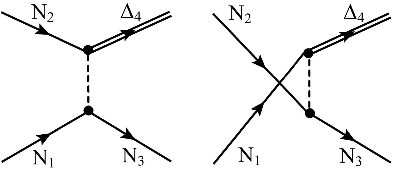
Figure B1.The left diagram is the direct term and the right is the exchange term of the Feynmann diagram.
$ {\cal{M}}^*={\cal{M}}_d^{*\pi}-{\cal{M}}_e^{*\pi}+{\cal{M}}_d^{*\rho}-{\cal{M}}_e^{*\rho}, $
(B1) where
$ \begin{aligned}[b] {\cal{M}}_d^{*\pi} =\;& -i\frac{g_{\pi NN} g_{\pi N\Delta} I_d }{ m_{\pi}^{2}( Q^{*2}_{d}- m_{\pi}^{2})}[\bar{\Psi}(p_3^* ) \gamma_{\mu}\gamma_5 Q_{d}^{*\mu} \Psi(p_1^*)]\\ & \times[\bar{\Delta}_{\nu} (p_4^* ) Q_d^{*\nu} \Psi(p_2^* )] \end{aligned} $
(B2) $ \begin{aligned}[b] {\cal{M}}_d^{*\rho} =\;& i\frac{\Gamma_{\rho NN} g_{\rho N\Delta}I_d}{m_{\rho} }[\bar{\Psi}(p_3^* ) \gamma_{\mu} \Psi(p_1^* )] \\ & \times\frac{g^{\mu\tau}-Q_d^{*\mu} Q_d^{*\tau}/m^{2}_{\rho}}{Q_d^{*2}-m^{2}_{\rho}}\\ & \nonumber \times[\bar{\Delta}_{\sigma} (p_4^* ) \gamma_{\lambda} \gamma_{5} (Q_d^{*\lambda} \delta_{\sigma\tau}-Q_d^{*\sigma} \delta_{\lambda\tau}) \Psi(p_2^* )]\; . \end{aligned} $
(B3) For the direct term,
$ Q_{d}^{*\mu}=p_{3}^{*\mu}-p_{1}^{*\mu} $ , while the exchange term$ {\cal{M}}^*_e $ is obtained by swapping$ p_{1}^{*\mu}\longleftrightarrow p_{2}^{*\mu} $ and$ Q_{e}^{*\mu}=p_{3}^{*\mu}-p_{2}^{*\mu} $ . The isospin factors$ I_d $ ,$ I_e $ are given in Ref. [10].The in-medium
$ NN\rightarrow N\Delta $ cross section is the averaged two-body cross section, taking into account the mass distribution of the ∆ resonance as a short-lived state. It can be expressed as:$ \sigma^*_{NN\rightarrow N\Delta}=\int_{m^*_{\Delta,\text{min}}}^{m^*_{\Delta,\text{max}}} dm^*_{\Delta}f(m^*_{\Delta})\tilde{\sigma}^*(m^*_{\Delta}), $
(B4) where
$ \tilde{\sigma}^*( m^*_{\Delta}) $ is the in-medium elementary two-body cross section. In the center-of-mass frame of colliding nucleons, it reads$ \tilde{\sigma}^*( m^*_{\Delta}) =\frac{1}{64\pi^2}\int \frac{|{\bf{p}}^{*}_{\text{out, c.m.}}|}{\sqrt{s^*_{\text{in}}}\sqrt{s^*_{\text{out}}}|{\bf{p}}^{*}_{\text{in, c.m.}}|} \overline{|{\cal{M}}^*|^2} d\Omega, $
(B5) where
$ {\bf{p}}^{*}_{\text{in, c.m.}} $ and$ {\bf{p}}^{*}_{\text{out, c.m.}} $ are the momenta of incoming (1 and 2) and outgoing particles (3 and 4), and$ s^*_{\text{in}}=(p^*_1+p^*_2)^2 $ , and$ s^*_{\text{out}}=(p^*_3+p^*_4)^2 $ .Here
$ \overline{|{\cal{M}}^*|^2}=\dfrac{1}{(2s_{1}+1)(2s_2+1)}\sum\limits_{s_{1}s_{2}s_{3}s_{4}}|{\cal{M}}^*|^2 $ is,$ \begin{aligned}[b]& \sum\limits_{s_{1}s_{2}s_{3}s_{4}}|{\cal{M}}^*|^2 \\ =\;&\sum\limits_{s_{1}s_{2}s_{3}s_{4}} \{ |{\cal{M}}_d^{*\pi}|^2-{\cal{M}}_d^{*\pi \dagger}{\cal{M}}_e^{*\pi}-{\cal{M}}_e^{*\pi \dagger}{\cal{M}}_d^{*\pi}+|{\cal{M}}_e^{*\pi}|^2\\ &+|{\cal{M}}_d^{*\rho}|^2-{\cal{M}}_d^{*\rho \dagger}{\cal{M}}_e^{*\rho}-{\cal{M}}_e^{*\rho \dagger}{\cal{M}}_d^{*\rho}+|{\cal{M}}_e^{*\rho}|^2 \\& +{\cal{M}}_d^{*\pi \dagger}{\cal{M}}_d^{*\rho}-{\cal{M}}_d^{*\pi \dagger}{\cal{M}}_e^{*\rho}-{\cal{M}}_e^{*\pi \dagger}{\cal{M}}_d^{*\rho}+{\cal{M}}_e^{*\pi \dagger}{\cal{M}}_e^{*\rho} \\& +{\cal{M}}_d^{*\rho \dagger}{\cal{M}}_d^{*\pi}-{\cal{M}}_d^{*\rho \dagger}{\cal{M}}_e^{*\pi}-{\cal{M}}_e^{*\rho \dagger}{\cal{M}}_d^{*\pi}+{\cal{M}}_e^{*\rho \dagger}{\cal{M}}_e^{*\pi}\}. \end{aligned} $
(B6) where the
$ {\cal{M}}^* $ -matrix is from exchange byπandρmesons, and the detail calculations can be found in Ref. [27]. Here, we show the calculation of$ \sum\limits_{s_{1}s_{2}s_{3}s_{4}} |{\cal{M}}_d^{*\pi}|^2 $ as an example in the following:$ \begin{aligned}[b]& \sum\limits_{s_{1}s_{2}s_{3}s_{4}} |{\cal{M}}_d^{*\pi}|^2 =\left(\frac{g_{\pi NN} g_{\pi N\Delta} I_d }{ m_{\pi}^{2}( Q^{*2}_{d}- m_{\pi}^{2})}\right)^2\\& \times\sum\limits_{s_{1}s_{2}s_{3}s_{4}}[\Psi(p_1^*)\bar{\Psi}(p_1^* ) \gamma_{\mu}\gamma_5 Q_{d}^{*\mu} \Psi(p_3^*)\bar{\Psi}(p_3^* )\gamma_{\sigma}\gamma_5 Q_{d}^{*\sigma}]\\& \times[\Psi(p_2^* )\bar{\Psi} (p_2^* ) Q_d^{*\nu} \Delta_{\nu} (p_4^* )\bar{\Delta}_{\tau} (p_4^* ) Q_d^{*\tau}]\\ =\;&\left(\frac{g_{\pi NN} g_{\pi N\Delta} I_d }{ m_{\pi}^{2}( t^{*}- m_{\pi}^{2})}\right)^2\\& \times\frac{2 (m^*_{N_{1}} + m^{*}_{N_{3}})^2((m^{*}_{N_{1}} - m^{*}_{N_{3}})^2 - t^*)}{3 m^{*2}_{\Delta_{4}}}\\& \times\left((m^{*}_{\Delta_{4}}-m^{*}_{N_{2}})^2 - t^*\right) \left((m^{*}_{N_{2}} + m^{*}_{\Delta_{4}})^2 - t^*\right)^2 \end{aligned} $
(B7) where
$ t=Q^{*2}_{d} $ , for$ |{\cal{M}}_e^{*\pi}|^2 $ is$ N_{1}\longleftrightarrow N_{2} $ . In Eq. (B5),the key element for the calculation of the cross section is the energy-momentum conservation in terms of the incoming ($ p^\mu_{1,2} $ ) and outgoing momenta ($ p^\mu_{3,4} $ ) of the particles. From the viewpoint of kinetic momentum, the energy-momentum conservation can be written as:$ p^\mu_{1}+p^\mu_{2}= p^\mu_{3}+p^\mu_{4} $ can be expressed as$ p^{*\mu}_{1}+\Sigma^{*\mu}_{1}+ p^{*\mu}_{2}+\Sigma^{*\mu}_{2}= p^{*\mu}_{3}+\Sigma^{*\mu}_{3}+p^{*\mu}_{4}+\Sigma^{*\mu}_{4} $ ,$ p^{*\mu}_{1}+ p^{*\mu}_{2}= p^{*\mu}_{3}+p^{*\mu}_{4}-\Delta\Sigma^{\mu} $ , where$ \Delta\Sigma^{\mu}=\Sigma^{\mu}_{1}+\Sigma^{\mu}_{2}-\Sigma^{\mu}_{3}-\Sigma^{\mu}_{4} $ is the kinetic momentum change between the initial and final states. The change in effective energy is expressed as$ \Delta \Sigma^0=\Sigma^{0}_{1}+\Sigma^{0}_{2}-\Sigma^{0}_{3}-\Sigma^{0}_{4} $ , which is the same the formula in Ref. [27,54]. The similar issue also exists in the calculation of$ m^{*}_{\text{min}} $ ,$ m^{*}_{\text{max}} $ and$ \Gamma(m^{*}_{\Delta}) $ which are described in the following. Consequently,$ p^{*0}_1+p^{*0}_2 $ may differ from$ p^{*0}_3+p^{*0}_4 $ , and$ s^*_{in}\ne s^*_{out} $ in Eq. (B5), and they are related according to the following relationship,$ \sqrt{s}=\sqrt{s^*_{in}}+\Sigma^0_{N_1}+\Sigma^0_{N_2}=\sqrt{s^*_{out}}+\Sigma^0_{N_3}+\Sigma^0_{\Delta_4}. $
(B8) It is derived from
$ \begin{aligned}[b] s =\;& (p_{N_{1}}+p_{N_{2}})^2\\ =\;& (\sqrt{m^{*2}_{N_{1}}+{\bf{p}}^{*2}_{N_{1}}}+\sqrt{m^{*2}_{N_{2}}+{\bf{p}}^{*2}_{N_{2}}}+\Sigma^0_{N_1}+\Sigma^0_{N_2})^2\\ & -({\bf{p}}^*_{N_{1}}+{\bf{p}}^*_{N_2})^2 \\ =\;& (p_{N_{3}}+p_{\Delta_4})^2\\ =\;& (\sqrt{m^{*2}_{N_{3}}+{\bf{p}}^{*2}_{N_{3}}}+\sqrt{m^{*2}_{\Delta_4}+{\bf{p}}^{*2}_{\Delta_4}}+\Sigma^0_{N_3}+\Sigma^0_{\Delta_4})^2\\& -({\bf{p}}^*_{N_{3}}+{\bf{p}}^*_{\Delta_4})^2 \end{aligned} $
(B9) where
$ {\bf{p}}^*_{N_1}=-{\bf{p}}^*_{N_2} $ and$ {\bf{p}}^*_{N_3}=-{\bf{p}}^*_{\Delta_4} $ in the center-of-mass frame.The value of
$ m^*_{\Delta,\text{min}} $ in the cross-section formula is determined by the$ \Delta \rightarrow N+ \pi $ in isospin asymmetric nuclear matter as in Refs. [27,55], where both theNandπare at rest. Additionally, the modification of the scalar and vector self-energies in this isospin exchange process must also be taken into account. Thus,$ m^*_{\Delta,\text{min}}=m^*_{N}+m_\pi-\Delta\Sigma_d^0, $
(B10) with
$ \Delta\Sigma_d^0=\Sigma_\Delta^0-\Sigma_{N}^0 $ . The$ m^*_{\Delta,\text{max}} $ is evaluated from$ NN\to N\Delta $ for producingNand ∆ at rest. This leads to:$ m^*_{\Delta,\text{max}}=\sqrt{s}-m^*_{N_{3}}-\Sigma^0_{N_{3}}-\Sigma^0_{\Delta_4}. $
(B11) The in-medium ∆ mass distribution
$ f(m^*_\Delta) $ is another crucial component of in-medium$ NN\rightarrow N\Delta $ cross section, for which proper energy conservation is also required, as$ f(m^*_\Delta) $ is related to the$ \Delta\rightarrow N+\pi $ process in isospin asymmetric nuclear matter. In this paper, the spectral function of ∆ is taken from Ref. [24],$ f(m^*_{\Delta})=\frac{2}{\pi}\frac{m^{* 2}_{\Delta}\Gamma(m^{*}_{\Delta})}{(m^{*2}_{0,\Delta}-m^{*2}_{\Delta})^2+m^{*2}_{\Delta}\Gamma^2(m^{*}_{\Delta}) }. $
(B12) Here,
$ m^*_{0,\Delta} $ is the effective pole mass of ∆. The decay width$ \Gamma(m^*_\Delta) $ is taken as the parameterization form [24]$ \Gamma(m^{*}_{\Delta})= \Gamma_{0}\frac{q^{3}(m^{* }_{\Delta},m^*_N,m^*_\pi)}{q^{3}(m^{*}_{0,\Delta},m^*_N,m^*_\pi)}\frac{q^{3}(m^{*}_{0,\Delta},m^*_N,m^*_\pi)+\eta^2}{q^{3}(m^{* }_{\Delta},m^*_N,m^*_\pi)+\eta^2}\frac{m^{*}_{0,\Delta}}{m^{*}_{\Delta}}, $
(B13) where
$ q(m^{*}_\Delta,m^*_{N},m^*_\pi)= \sqrt{\frac{\left((m^*_\Delta+\Sigma^{0}_{\Delta}-\Sigma^{0}_{N})^2+m_{N}^{*2}-m_{\pi}^{* 2}\right)^2} {4(m^{*}_\Delta+\Sigma^{0}_{\Delta}-\Sigma^{0}_{N})^2}-m_{N}^{*2}}. $
(B14) The coefficients of
$ \Gamma_0 $ =0.118 GeV andη=0.2 GeV/care used in the above parameterization formula.The form factors are adopted to effectively consider the contributions from high-order terms and the finite size of baryons [10,56], which read
$ F_N (t^*)=\frac{\Lambda_N^2}{\Lambda_N^2-t^*} exp\left(-b\sqrt{s^*-4m_N^{* 2}}\right) $
(B15) $ F_{\Delta}(t^*)=\frac{\Lambda_{\Delta}^2}{\Lambda_{\Delta}^2-t^*}. $
(B16) Here
$ F_N (t^* ) $ is the form factor for nucleon-meson-nucleon, and$ F_\Delta (t^*) $ for nucleon-meson-∆ coupling,b=0.046 GeV−1for both$ \rho NN $ and$ \pi NN $ coupling. The cutoff parameter$ \Lambda_{\pi N N}\approx 1 $ GeV,$ \Lambda_{\rho N N} $ and$ \Lambda_{\pi N \Delta} $ are determined by best fitting the data of$ NN\rightarrow N\Delta $ cross section in free space ranging from$ \sqrt{s} $ =2.0 to 5 GeV [45]. Here,$ \Lambda_{\rho N \Delta} $ is determined based on the relationship$ \Lambda_{\rho N \Delta}=\Lambda_{\rho NN}\dfrac{\Lambda_{\pi N\Delta}}{\Lambda_{\pi NN}} $ as in [10]. Concerning the coupling constant$ g_{\rho N\Delta} $ , we use$ g_{\rho N\Delta}\approx\dfrac{\sqrt{3}}{2} \Gamma_{\rho NN} \dfrac{m_{\rho}}{m_N} $ which are derived from the static quark model [10]. The cutoff parameters used in calculations of in-medium$ NN\rightarrow N\Delta $ cross sections are listed inTable C1in Appendix C.
-
For the coupling constant parameters of
$ g_{m\Delta\Delta} $ (where$ m=\sigma, \omega, \rho, \delta $ ), we adopt$ g_{m}=g_{m\Delta\Delta}=g_{mNN} $ consistent with the approach used in many studies involving transport models [11,24,26]. The parameters used in the effective Lagrangian,$ g_{\pi NN} $ =1.008,$ g_{\pi N\Delta} $ =2.202,$ m_{\pi} $ =138 MeV,$ m_{N} $ =939 MeV,$ m_{0,\Delta} $ =1232 MeV.Model $E_0$ $\rho_{0}$ $K_0$ J L $K_{sym}$ $m^{*}_{N}/m_{N}$ $m^{*}_{0,\Delta}/m_{0,\Delta}$ $\Lambda_{\pi N\Delta}$ Nonlinear models E [57] −16.35 0.150 210.95 38.58 124.69 133.52 0.578 0.679 417 ER [57] −16.25 0.149 215.91 39.41 126.63 128.12 0.582 0.682 416 NL1 [58] −16.42 0.152 212.35 43.54 140.37 143.39 0.572 0.674 415 NL3 [59] −16.24 0.148 269.91 37.34 118.32 100.53 0.596 0.692 417 NL3-II [59] −16.26 0.149 270.62 37.67 119.57 103.19 0.593 0.690 417 NL3*[60] −16.31 0.150 258.76 38.70 122.72 105.72 0.594 0.690 417 NL4 [61] −16.16 0.148 273.33 36.34 115.31 100.41 0.595 0.692 417 NLC [62] −15.77 0.148 221.76 35.23 108.52 76.14 0.633 0.720 417 NLB1 [58] −15.80 0.162 276.73 32.94 102.12 75.61 0.621 0.711 420 NLB2 [58] −15.80 0.162 239.96 32.93 110.57 157.15 0.557 0.662 421 NLRA1 [63] −16.15 0.147 284.42 36.44 115.31 95.56 0.597 0.693 417 NLS [64] −16.45 0.150 262.98 42.08 131.61 94.27 0.604 0.698 415 P-067 [65] −16.31 0.160 245.72 41.80 124.81 48.93 0.665 0.745 416 P-070 [65] −16.25 0.160 228.23 41.04 119.74 26.04 0.702 0.773 416 P-075 [65] −16.51 0.170 253.33 42.17 119.16 −2.19 0.755 0.813 416 P-080 [65] −15.84 0.160 251.71 39.28 108.78 −14.06 0.800 0.847 416 GL1 [66] −16.30 0.153 200.08 32.50 94.68 33.08 0.700 0.772 418 GL2 [66] −16.31 0.153 199.92 32.50 91.52 8.74 0.750 0.810 418 GL3 [66] −16.31 0.153 199.87 32.50 89.03 −8.43 0.800 0.848 417 GL4 [66] −16.31 0.153 249.88 32.50 94.31 25.23 0.700 0.772 418 GL5 [66] −16.31 0.153 249.81 32.50 91.19 2.63 0.750 0.810 418 GL6 [66] −16.31 0.153 249.90 32.50 88.73 −12.93 0.800 0.848 417 GL7 [66] −16.30 0.153 299.99 32.50 93.94 17.94 0.700 0.772 418 GL8 [66] −16.31 0.153 299.84 32.50 90.86 −2.91 0.750 0.810 418 GL82 [67] −16.00 0.145 285.41 36.22 101.28 −8.06 0.773 0.827 416 GL9 [66] −16.31 0.153 299.89 32.50 88.44 −16.84 0.800 0.848 417 GM1 [68] −16.34 0.153 299.85 32.50 93.96 17.96 0.700 0.772 418 GM2 [68] −16.31 0.153 299.94 32.50 89.34 −11.99 0.780 0.832 418 GM3 [68] −16.30 0.153 239.93 32.50 89.71 −6.46 0.780 0.832 418 GPS1 [69] −15.98 0.150 250.46 32.52 88.96 −12.54 0.800 0.848 417 GPS2 [69] −15.96 0.150 300.67 32.52 88.66 −16.42 0.800 0.848 417 NLρA [29] −16.00 0.160 240.16 30.34 84.52 3.38 0.750 0.809 419 NLρB [29] −16.30 0.148 271.55 33.70 106.87 95.85 0.600 0.695 418 RMF301 [70] −16.30 0.153 253.79 32.50 89.87 −6.24 0.775 0.829 418 RMF302 [70] −16.30 0.153 249.64 32.50 89.65 −7.35 0.780 0.832 418 RMF303 [70] −16.30 0.153 248.80 32.50 89.61 −7.57 0.781 0.833 418 RMF304 [70] −16.30 0.153 247.97 32.50 89.57 −7.78 0.782 0.834 418 RMF305 [70] −16.30 0.153 246.30 32.50 89.49 −8.21 0.784 0.835 418 RMF306 [70] −16.30 0.153 244.62 32.50 89.40 −8.63 0.786 0.837 418 RMF307 [70] −16.30 0.153 243.77 32.50 89.36 −8.83 0.787 0.838 418 RMF308 [70] −16.30 0.153 242.94 32.50 89.32 −9.04 0.788 0.838 418 RMF309 [70] −16.30 0.153 241.24 32.50 89.24 −9.45 0.790 0.840 418 RMF310 [70] −16.30 0.153 238.68 32.50 89.12 −10.04 0.793 0.842 418 RMF311 [70] −16.30 0.153 237.82 32.50 89.08 −10.24 0.794 0.843 417 RMF312 [70] −16.30 0.153 236.96 32.50 89.04 −10.43 0.795 0.844 417 RMF313 [70] −16.30 0.153 235.24 32.50 88.96 −10.82 0.797 0.845 417 RMF314 [70] −16.30 0.153 234.39 32.50 88.92 −11.01 0.798 0.846 417 RMF315 [70] −16.30 0.153 233.94 32.50 88.90 −11.10 0.799 0.846 417 RMF316 [70] −16.30 0.153 233.51 32.50 88.88 −11.20 0.799 0.847 417 RMF317 [70] −16.30 0.153 232.65 32.50 88.84 −11.38 0.800 0.848 417 RMF401 [70] −16.31 0.153 229.87 32.50 93.78 23.04 0.710 0.779 418 RMF402 [70] −16.31 0.153 231.87 32.50 93.77 22.74 0.710 0.779 418 RMF403 [70] −16.31 0.153 229.88 32.50 93.12 18.06 0.720 0.787 418 RMF404 [70] −16.47 0.153 230.42 32.50 93.14 17.86 0.720 0.786 418 RMF405 [70] −16.31 0.153 233.88 32.50 93.09 17.50 0.720 0.787 418 RMF406 [70] −16.31 0.153 233.92 32.50 89.75 −5.80 0.780 0.832 418 RMF407 [70] −16.31 0.153 229.89 32.50 92.50 13.42 0.730 0.794 418 RMF408 [70] −16.31 0.153 231.89 32.50 92.48 13.15 0.730 0.794 418 RMF409 [70] −16.31 0.153 233.89 32.50 92.47 12.88 0.730 0.794 418 RMF410 [70] −16.31 0.153 235.89 32.50 92.45 12.62 0.730 0.794 418 RMF411 [70] −16.31 0.153 229.90 32.50 91.90 9.09 0.740 0.802 418 RMF412 [70] −16.31 0.153 231.90 32.50 91.88 8.84 0.740 0.802 418 RMF413 [70] −16.31 0.153 233.90 32.50 91.87 8.58 0.740 0.802 418 RMF414 [70] −16.31 0.153 235.90 32.50 91.86 8.33 0.740 0.802 418 RMF415 [70] −16.30 0.153 229.91 32.50 91.33 5.06 0.750 0.809 418 RMF416 [70] −16.30 0.153 231.91 32.50 91.31 4.82 0.750 0.809 418 RMF417 [70] −16.30 0.153 233.91 32.50 91.30 4.58 0.750 0.809 418 RMF418 [70] −16.30 0.153 235.91 32.50 91.29 4.34 0.750 0.809 418 RMF419 [70] −16.31 0.153 229.91 32.50 90.79 1.31 0.760 0.817 418 RMF420 [70] −16.31 0.153 231.91 32.50 90.77 1.09 0.760 0.817 418 RMF421 [70] −16.31 0.153 233.91 32.50 90.76 0.86 0.760 0.817 418 RMF422 [70] −16.31 0.153 229.92 32.50 90.27 −2.17 0.770 0.825 418 RMF423 [70] −16.31 0.153 231.91 32.50 90.26 −2.38 0.770 0.825 418 RMF424 [70] −16.30 0.153 245.93 32.50 89.21 −9.88 0.790 0.840 418 RMF425 [70] −16.30 0.153 247.94 32.50 89.20 −10.06 0.790 0.840 418 RMF426 [70] −16.30 0.153 249.94 32.50 89.19 −10.24 0.790 0.840 418 RMF427 [70] −16.30 0.153 235.94 32.50 88.83 −11.67 0.800 0.848 417 RMF428 [70] −16.30 0.153 237.94 32.50 88.81 −11.85 0.800 0.848 417 RMF429 [70] −16.30 0.153 239.94 32.50 88.80 −12.02 0.800 0.848 417 RMF430 [70] −16.30 0.153 241.94 32.50 88.79 −12.19 0.800 0.848 417 RMF431 [70] −16.30 0.153 243.94 32.50 88.78 −12.36 0.800 0.848 417 RMF432 [70] −16.30 0.153 245.94 32.50 88.77 −12.53 0.800 0.848 417 RMF433 [70] −16.30 0.153 247.94 32.50 88.75 −12.70 0.800 0.848 417 RMF434 [70] −16.30 0.153 249.94 32.50 88.74 −12.87 0.800 0.848 417 Q1 [71] −16.10 0.148 242.19 36.46 115.77 105.77 0.597 0.693 417 SMFT2 [72] −13.85 0.162 210.02 17.37 52.72 60.28 0.656 0.738 430 S271 [38] −16.24 0.148 270.94 35.03 101.91 22.28 0.700 0.771 417 SRK3M5 [73] −16.00 0.150 299.95 23.50 82.46 146.79 0.550 0.657 425 DJM [72] −14.81 0.172 245.71 20.23 63.03 32.62 0.569 0.671 430 HD [74] −16.22 0.177 283.50 35.67 105.86 44.51 0.666 0.746 419 MS1 [75] −15.75 0.148 249.97 35.00 106.76 38.56 0.600 0.695 418 MS3 [76] −15.75 0.148 247.80 34.91 102.11 −0.10 0.601 0.696 418 NLSV1 [77] −16.26 0.149 269.49 37.28 114.61 58.91 0.613 0.705 417 NLSV2 [77] −16.24 0.147 293.95 36.84 111.78 39.60 0.618 0.709 417 TM1 [78] −16.26 0.145 279.55 36.84 110.61 33.55 0.635 0.722 416 PK1 [79] −16.22 0.148 283.39 37.61 115.78 55.17 0.605 0.700 417 Z271 [38] −16.24 0.148 270.96 33.30 91.02 −16.40 0.800 0.848 417 hybrid [80] −16.24 0.148 228.75 37.24 118.41 110.50 0.596 0.692 417 Z271*[81] −16.24 0.148 268.69 40.18 83.52 −197.69 0.800 0.848 413 HC [74] −15.75 0.169 233.88 31.06 58.60 −98.75 0.679 0.756 417 XS [76] −16.30 0.148 228.11 31.78 54.85 −28.76 0.601 0.696 410 BKA20 [82] −16.09 0.146 236.89 32.24 75.39 −15.04 0.642 0.727 412 BKA22 [82] −16.08 0.147 223.09 33.13 78.67 −8.84 0.608 0.701 410 BKA24 [82] −16.13 0.147 225.97 34.18 84.77 −14.95 0.603 0.698 413 FSUGOLD [83] −16.28 0.148 228.56 32.54 60.38 −51.45 0.611 0.703 413 FSUGOLD4 [84] −16.53 0.148 228.95 31.47 51.98 −16.12 0.610 0.703 410 FSUGOLD5 [84] −16.92 0.148 229.53 30.56 45.66 23.28 0.610 0.703 413 FSUGZ00 [85] −16.03 0.149 241.74 31.47 62.27 −3.22 0.605 0.699 410 FSUGZ03 [85] −16.07 0.147 230.73 31.50 63.86 −11.75 0.603 0.698 410 FSUGZ06 [85] −16.05 0.146 226.48 31.22 62.53 −24.49 0.607 0.700 410 IU-FSU [86] −16.40 0.155 233.39 31.34 47.35 28.99 0.609 0.702 410 NL3V1 [87] −16.24 0.148 269.60 36.01 101.08 0.62 0.596 0.692 416 NL3V2 [87] −16.24 0.148 269.60 34.93 87.64 −46.25 0.596 0.692 416 NL3V3 [87] −16.24 0.148 269.60 34.43 81.97 −56.29 0.596 0.692 416 NL3V4 [87] −16.24 0.148 269.60 33.98 76.87 −60.12 0.596 0.692 415 NL3V5 [87] −16.24 0.148 269.60 33.12 68.15 −53.40 0.596 0.692 415 NL3V6 [87] −16.24 0.148 269.60 32.35 61.05 −34.30 0.596 0.692 414 S271V1 [87] −16.24 0.148 270.98 35.73 95.92 −44.06 0.700 0.771 416 S271V2 [87] −16.24 0.148 270.98 35.05 86.87 −90.33 0.700 0.771 416 S271V3 [87] −16.24 0.148 270.98 34.42 78.86 −120.99 0.700 0.771 416 S271V4 [87] −16.24 0.148 270.98 33.82 71.75 −139.52 0.700 0.771 415 S271V5 [87] −16.24 0.148 270.98 33.27 65.44 −148.63 0.700 0.771 415 S271V6 [87] −16.24 0.148 270.98 32.74 59.81 −150.45 0.700 0.771 415 Z271S1 [87] −16.24 0.148 270.95 34.95 86.86 −64.86 0.800 0.848 415 Z271S2 [87] −16.24 0.148 270.95 34.07 76.62 −92.28 0.800 0.848 415 Z271S3 [87] −16.24 0.148 270.95 33.27 67.81 −104.57 0.800 0.848 414 Z271S4 [87] −16.24 0.148 270.95 32.53 60.18 −106.04 0.800 0.848 414 Z271S5 [87] −16.24 0.148 270.95 31.84 53.57 −99.82 0.800 0.848 413 Z271S6 [87] −16.24 0.148 270.95 31.20 47.80 −88.22 0.800 0.848 412 Z271V1 [87] −16.24 0.148 270.95 35.34 90.86 −66.36 0.800 0.848 416 Z271V2 [87] −16.24 0.148 270.95 34.80 83.61 −104.83 0.800 0.848 416 Z271V3 [87] −16.24 0.148 270.95 34.54 80.23 −120.38 0.800 0.848 415 Z271V4 [87] −16.24 0.148 270.95 34.28 76.99 −133.75 0.800 0.848 415 Z271V5 [87] −16.24 0.148 270.95 34.04 73.90 −145.14 0.800 0.848 415 Z271V6 [87] −16.24 0.148 270.95 33.80 70.94 −154.73 0.800 0.848 415 G1 [71] −16.14 0.153 215.34 38.51 123.30 97.03 0.633 0.721 417 G2 [71] −16.07 0.154 215.00 36.40 100.71 −7.48 0.664 0.744 416 G2*[81] −16.07 0.154 216.87 30.46 69.87 −21.86 0.663 0.743 413 TM1*[88] −16.33 0.145 281.13 36.87 101.72 −13.78 0.634 0.721 415 BSR1 [89] −16.02 0.148 239.60 31.03 59.39 12.92 0.605 0.699 410 BSR2 [89] −16.03 0.149 241.81 31.54 62.14 −2.87 0.605 0.699 410 BSR3 [89] −16.09 0.150 232.84 32.81 70.63 −7.45 0.604 0.698 410 BSR4 [89] −16.08 0.150 236.47 33.12 73.09 −20.92 0.607 0.700 412 BSR5 [89] −16.12 0.151 237.33 34.51 83.51 −14.00 0.607 0.700 413 BSR6 [89] −16.13 0.149 233.88 35.57 85.54 −49.59 0.602 0.697 414 BSR7 [89] −16.18 0.149 229.76 37.19 98.93 −17.04 0.602 0.697 415 BSR8 [89] −16.04 0.147 231.44 31.09 60.29 −0.68 0.606 0.699 410 BSR9 [89] −16.08 0.147 230.70 31.57 63.76 −11.42 0.603 0.698 410 BSR10 [89] −16.07 0.147 224.90 32.65 70.64 −16.62 0.601 0.696 410 BSR11 [89] −16.08 0.147 227.98 33.73 78.89 −24.71 0.605 0.699 412 BSR12 [89] −16.10 0.147 230.14 33.93 77.73 −44.28 0.608 0.701 414 BSR13 [89] −16.13 0.147 227.25 35.77 90.94 −41.62 0.604 0.698 415 BSR14 [89] −16.18 0.147 233.29 36.24 93.64 −41.83 0.609 0.702 415 BSR15 [89] −16.03 0.146 229.14 31.04 61.96 −21.36 0.607 0.700 410 BSR16 [89] −16.05 0.146 226.57 31.29 62.45 −24.16 0.607 0.700 410 BSR17 [89] −16.05 0.146 219.62 31.92 67.28 −31.57 0.609 0.702 410 BSR18 [89] −16.05 0.146 221.63 32.76 72.69 −42.25 0.606 0.700 412 BSR19 [89] −16.08 0.147 222.06 33.83 79.58 −50.19 0.608 0.701 414 BSR20 [89] −16.09 0.146 222.69 34.51 87.97 −39.86 0.606 0.700 415 BSR21 [89] −16.12 0.145 219.47 35.92 92.86 −45.94 0.602 0.697 415 SVI-1 [90] −16.30 0.149 261.34 36.94 116.12 95.11 0.617 0.708 417 SVI-2 [90] −16.31 0.149 273.61 37.13 116.39 91.95 0.620 0.710 417 SIG-OM [91] −16.31 0.149 262.58 36.91 111.62 40.96 0.623 0.713 417 NL $\rho\delta$ A [29]−16.00 0.160 240.16 30.71 102.67 127.37 0.750 0.809 410 NL $\rho\delta$ B [29]−16.30 0.148 271.55 34.06 138.90 398.27 0.600 0.695 410 Density-dependent models DD-ME2 [52] −16.14 0.152 251.27 32.31 51.27 −87.22 0.572 0.674 410 DD-ME1 [92] −16.23 0.152 243.84 33.06 55.43 −101.03 0.578 0.678 410 TW99 [93] −16.25 0.153 240.16 32.76 55.31 −124.69 0.555 0.661 412 DD-F [94] −16.04 0.147 222.87 31.62 55.97 −139.71 0.556 0.662 413 DD2 [95] −16.03 0.149 242.41 31.67 55.03 −93.21 0.563 0.667 412 DD [96] −16.02 0.149 239.88 31.64 55.97 −95.29 0.565 0.668 412 PKDD [79] −16.27 0.150 261.94 36.79 90.20 −80.54 0.571 0.673 415 DDMEδ[30] −16.08 0.152 219.59 32.34 52.80 −118.13 0.609 0.702 416 DDRH $\rho\delta$ [31]−16.25 0.153 240.16 25.09 47.81 81.15 0.555 0.661 417 Point-coupling models FA3 [50] −16.02 0.152 275.90 29.69 29.08 −275.05 0.676 0.753 430 FA4 [50] −16.09 0.152 293.79 29.77 30.65 −257.83 0.680 0.756 430 FZ3 [50] −15.93 0.152 297.75 29.96 33.78 −262.69 0.742 0.803 430 VZ3 [50] −16.04 0.148 282.09 34.03 121.49 151.25 0.626 0.715 430 PC-F1 [51] −16.18 0.151 255.20 37.78 117.15 74.68 0.610 0.703 430 PC-F3 [51] −16.18 0.151 254.99 38.26 118.57 74.74 0.610 0.703 430 Table C1.The saturation properties of all RMF models are used in this work. Excepting for
$m^{*}_{N}/m_{N}$ and$m^{*}_{0,\Delta}/m_{0,\Delta}$ in dimensionless, and$\rho_{0}$ in fm−3, all entries are in MeV. All$\Lambda_{\rho NN}=1000$ MeV, except for$\Lambda_{\rho NN}=798$ , 650 and 580 MeV for FSUGOLD5, DDMEδand DDRH$\rho\delta$ .


 DownLoad: