SU(3) analysis forB(E2) anomaly

Understanding the deformations of nuclei and how they change, whether continuously or abruptly, is one of the fundamental problems in nuclear structure. Quadrupole deformations are the most significant. A geometrical model with deformation variablesβandγprovides a good description, whereβrepresents the degree of deviation from the spherical shape andγrepresents the angle that describes the triaxial deformation. Fifty years ago, the interacting boson model (IBM) was proposed [1,2], which is an algebraic model for describing the collective excitations (deformations) in the nuclear structure. For the simplest case, only thesanddbosons with angular momentum $ L = 0 $ and $ L = 2 $ , respectively, are considered to construct the Hamiltonian, which features theU(6) symmetry. Four dynamical symmetry limits exist:U(5) symmetry (spherical shape),SU(3) symmetry (prolate shape),O(6) symmetry (γ-soft rotation), and $ \overline{\rm{\mathit{SU}(3)}} $ symmetry (oblate shape) [3]. Shape phase transitions between different shapes can also be studied using this model [4−18]. Thus, the IBM provides an efficient theoretical framework to describe various deformations of nuclei and their collective excitation behaviors, and it has a broad impact in the field of nuclear structure.

Although the IBM is self-consistent for describing various quadrupole deformations, some experimental anomalies appear to be indescribable by previous model Hamiltonians, such as theB(E2) anomaly [19−22] and Cd puzzle [23−28]. In theB(E2) anomaly, the ratio $ E_{4/2} = E_{4_{1}^{+}}/E_{2_{1}^{+}} $ of the energies for the $ 4_{1}^{+} $ , $ 2_{1}^{+} $ states is greater than 2.0 (a feature for the collective excitations). However, the ratio $ B_{4/2} = B(E2;4_{1}^{+}\rightarrow 2_{1}^{+})/B(E2;2_{1}^{+}\rightarrow 0_{1}^{+}) $ of theE2 transitions $ B(E2;4_{1}^{+}\rightarrow 2_{1}^{+}) $ and $ B(E2;2_{1}^{+}\rightarrow 0_{1}^{+}) $ can be much smaller than 1.0 (a traditional signal for non-collective behaviors), which cannot be possibly explained by previous theories on nuclear structure [19−22]. Regarding the Cd puzzle, the experimental data did not confirm the phonon excitations of the spherical nucleus [23−27], thereby questioning their existence [28]. Experimentally, theB(E2) anomaly and Cd puzzle can occur in adjacent nuclei, such as $ ^{72-76} {\rm{Zn}}$ [29−31], and even in a single nucleus, such as $ ^{114} {\rm{Te}}$ [32,33]. Therefore, they may have a common origin.

Moreover, it was found that nuclei previously considered to have a prolate shape should be rigid triaxial [34−36], making previous IBM descriptions not particularly convenient. In such descriptions, the spectra of the prolate (SU(3) symmetry limit) and oblate ( $ \overline{\rm{\mathit{SU}(3)}} $ symmetry limit) shapes are the same [3]. However, this mirror symmetry cannot be found in realistic nuclei [37].

Therefore, it is necessary to further generalize upon the existing models. Recently, an extension of the interacting boson model withSU(3) higher-order interactions (SU3-IBM) was proposed to resolve the aforementioned various anomalies. In the SU3-IBM, by introducing theSU(3) third-order and fourth-order interactions, theSU(3) symmetry limit can describe both prolate (SU(3) second Casimir operator $ -\hat{C}_2[{\mathit{SU}(3)}] $ ) and oblate ( $ \hat{C}_3[{\mathit{SU}(3)}] $ ) shapes as well as various rigid triaxial shapes (combinations of $ -\hat{C}_{2}[ {\mathit{SU}(3)}] $ , $ \hat{C}_{3}[ {\mathit{SU}(3)}] $ , and $ \hat{C}_{2}^{2}[ {\mathit{SU}(3)}] $ ), and even dynamical effects independent of the ground state. Thus, theSU(3) symmetry plays a more important role.

Through detailed analysis, it was found that this model can better describe the collective behaviors of atomic nuclei. In particular, it can describe theB(E2) anomaly and Cd puzzle [38,39]. Although theB(E2) anomaly cannot be described by previous nuclear theories [19−22], many possible explanations have been proposed in the SU3-IBM and other extended IBM theories [40−48]. The spherical-like spectra for resolving the Cd puzzle were actually found in $ ^{106} {\rm{Pd}}$ [49]. The SU3-IBM can also be used to explain the prolate-oblate shape asymmetric transitions in the Hf-Hg region [50−52], to better describe theγ-soft behaviors in $ ^{196} {\rm{Pt}}$ [53], to describe the E(5)-like spectra in $ ^{82} {\rm{Kr}}$ [54], and to explain the unique boson number odd-even phenomenon in $ ^{196-204} {\rm{Hg}}$ [55], which was first reported in Ref. [51]. Furthermore, it can well describe the rigid triaxiality in $ ^{166} {\rm{Er}}$ [56]. Recently, the shape phase transition from the newγ-soft phase to the prolate shape was also reported, with $ ^{108} {\rm{Pd}}$ being the critical nucleus [57]. These results have overturned our traditional understanding of nuclear structure, as they have captured nearly all shape patterns and provided new collective patterns for describing various anomalous behaviors.

Based on previous studies [40−48], discussions on the mechanisms underlying theB(E2) anomaly continue. To date, many possible explanations have been proposed for this anomaly. More fundamental discussions could clarify certain key parts. We introduce the concept ''SU(3) analysis,'' which is applied to re-analyze the results obtained in these studies within theSU(3) symmetry limit. We remove the non-SU(3) symmetry parts of the Hamiltonian to discuss whether the remainingSU(3) symmetry part can have theB(E2) anomaly ( $ B(E2;4_{1}^{+}\rightarrow 2_{1}^{+}) = 0 $ ). If this is the case, it may be the reason for the emergence of theB(E2) anomaly in the original Hamiltonian. For the remainingSU(3) symmetry part, we assume that the parameter in front of theSU(3) third-order interaction $ [L\times Q \times L]^{(0)} $ varies, and the partial low-lying levels and values of $ B(E2;2_{1}^{+}\rightarrow 0_{1}^{+}) $ , $ B(E2;4_{1}^{+}\rightarrow 2_{1}^{+}) $ and $ B(E2;6_{1}^{+}\rightarrow 4_{1}^{+}) $ are analyzed. We found three new results: (1) The interaction $ [L\times Q \times L]^{(0)} $ is critical for theSU(3) anomaly, (2) level-crossing within theSU(3) symmetry limit is crucial for theSU(3) anomaly, and (3) not only the value of $ B(E2;4_{1}^{+}\rightarrow 2_{1}^{+}) $ but also those of $ B(E2;6_{1}^{+}\rightarrow 4_{1}^{+}) $ and $ B(E2;2_{1}^{+}\rightarrow 0_{1}^{+}) $ can be anomalous (these values can be 0). Thus,SU(3) analysis is a useful tool for identifying the real cause. We expect it can be used in future discussions on theB(E2) anomaly.

In the SU3-IBM, theU(5) symmetry andSU(3) symmetry limits are included (some bias towards theO(6) symmetry may be also required). In theSU(3) symmetry limit, theSU(3) second-order Casimir operator $ -\hat{C}_{2}[ {\mathit{SU}(3)}] $ can describe the prolate shape and theSU(3) third-order Casimir operator $ \hat{C}_{3}[ {\mathit{SU}(3)}] $ can describe the oblate shape, which is the fundamental difference from the previous IBM [52]. The rigid triaxial shape can be obtained by the combinations of the square of theSU(3) second-order Casimir operator $ \hat{C}_{2}^{2}[ {\mathit{SU}(3)}] $ and $ -\hat{C}_{2}[ {\mathit{SU}(3)}] $ , $ \hat{C}_{3}[ {\mathit{SU}(3)}] $ . Moreover, theSU(3) invariants $ [L\times Q \times L]^{(0)} $ and $ [(L \times Q)^{(1)}\times (L \times Q)^{(1)}]^{(0)} $ are necessary.

The Hamiltonian is as follows:

whereα,β,γ,δ,η,ζ,andξare fitting parameters; $ \hat{n}_{d} = d^{\dagger}\cdot \tilde{d} $ is thedboson number operator; $ \hat{Q} = [d^{\dagger}\times\tilde{s}+ s^{\dagger}\times \tilde{d}]^{(2)}-\dfrac{\sqrt{7}}{2}[d^{\dagger}\times \tilde{d}]^{(2)} $ is theSU(3) quadrupole operator; and $ \hat{L} = \sqrt{10}[d^{\dagger}\times \tilde{d}]^{(1)} $ is the angular momentum operator. The first four interactions determine the quadrupole shapes of the ground state of the nucleus and the positions of the $ 0^{+} $ states of the excited levels. The remaining three ones are dynamical interactions and can be used to change the features of the non- $ 0^{+} $ states.

The twoSU(3) Casimir operators are related with the quadrupole second- or third-order interactions as follows:

For a givenSU(3) irreducible representation $ (\lambda,\mu) $ , the eigenvalues of the two Casimir operators under the group chain $ \rm{\mathit{U}(6)}\supset\mathit{SU}(3)\supset\rm{\mathit{O}(3)} $ are expressed as

TheSU(3) irreducible representation $ (\lambda,\mu) $ can be related with the quadrupole deformation variablesβandγas

and

where $ \beta_{0} $ is a scale factor.

For understanding theB(E2) anomaly, theB(E2) values are necessary. The $ E2 $ operator is defined as

whereqis the boson effective charge. The evolutions of $ B(E2; 2_{1}^{+}\rightarrow 0_{1}^{+}) $ , $ B(E2; 4_{1}^{+}\rightarrow 2_{1}^{+}) $ , and $ B(E2; 6_{1}^{+}\rightarrow 4_{1}^{+}) $ values are discussed.

TheB(E2) anomaly cannot be explained by previous nuclear structure theories. However, in the extended IBM with higher-order interactions, it can be described using different approaches [40−48]. A key problem is to determine whether these explanations are related with theSU(3) symmetry. Evidently, these explanations must be considered in theSU(3) symmetry limit. To explain theB(E2) anomaly in realistic nuclei, the boson number operator $ \hat{n}_{d} $ is needed in some descriptions or theSU(3) quadrupole operator $ \hat{Q} $ is replaced by the generalized quadrupole operator $ \hat{Q}_{\chi} = [d^{\dagger}\times\tilde{s}+s^{\dagger}\times \tilde{d}]^{(2)}+\chi[d^{\dagger}\times \tilde{d}]^{(2)} $ (some bias towards theO(6) symmetry means $ \chi\neq -\dfrac{\sqrt{7}}{2} $ ). Thus, forSU(3) analysis, the $ \hat{n}_{d} $ interaction should be removed (hereα= 0), and $ \hat{Q}_{\chi} $ is replaced by $ \hat{Q} $ again (here $ \chi = -\dfrac{\sqrt{7}}{2} $ ). The non-SU(3) symmetry parts are removed. If these operations are feasible, theSU(3) analysis exists, which is important for understanding the emergence of theB(E2) anomaly. This analysis has been ignored in previous studies. In this study, we demonstrate that it is critical.

TheB(E2) anomaly implies that $ B_{4/2}<1.0 $ while $ E_{4/2}\geq 2.0 $ . These two quantities involve only $ 0_{1}^{+} $ , $ 2_{1}^{+} $ , and $ 4_{1}^{+} $ states; therefore, they are important for the success of any nuclear structure theories. This point is similar to the magic number in atomic nuclei, which is only related with the $ 0_{1}^{+} $ and $ 2_{1}^{+} $ states. It should be noticed that thisB(E2) anomaly was first theoretically reported in Ref. [58], but it is not consistent with the experimental data reported in Refs. [19−22], in which the $ B_{4/2} $ values are much smaller than 1.0, even reaching 0.33. We found that theB(E2) anomaly is a phenomenon as important as that of magic numbers. If a theory cannot explain theB(E2) anomaly, it is insufficient.

Through numerous careful calculations, we found that theSU(3) cubic interaction $ [L\times Q \times L]^{(0)} $ plays an important role in explaining theB(E2) anomaly. (Whether this relationship is unique is still unclear). Thus, when discussing the problem, we let the coefficientηof this interaction change and analyze the characteristics of theB(E2) anomaly.

Next, we discuss the first example usingSU(3) analysis.Fig. 1(a) shows the evolutional behaviors of the partial low-lying levels as a function ofηin theSU(3) symmetry limit in Ref. [40]. This is the first successful explanation for theB(E2) anomaly of realistic nucleus $ ^{170} {\rm{Os}}$ . The boson number is $ N = 9 $ . In Ref. [40], the parameters are $ \alpha = 302.4 $ keV, $ \beta = -30.09 $ keV, $ \gamma = 3.79 $ keV, $ \delta = 0.0 $ keV, $ \eta = -10.38 $ keV, $ \zeta = 0.0 $ keV, and $ \xi = 18.66 $ keV. ForSU(3) analysis, let $ \alpha = 0 $ . The ground state is a prolate shape withSU(3) irrep (18,0). In that previous study, the twoSU(3) third-order interactions were considered, unlike the two four-order interactions. FromFig. 1(a), we can see that whenηvaries from 0 to −20.76 keV (the middle point $ \eta = -10.38 $ keV is the parameter used in Ref. [40]), the red dashed line of the $ 4_{1}^{+} $ state intersects with that of another $ 4^{+} $ state at $ \eta = -6.45 $ keV (the crossover point is marked by the black circle, and the latter ones are also the same). In Ref. [40], it was reported that the $ 4^{+} $ state in theSU(3) irrep (10,4) becomes lower than the $ 4^{+} $ state in theSU(3) irrep (18,0). InFig. 1(a), we observe new features that were not observed in previous studies. The $ 6_{1}^{+} $ state intersects with the other $ 6^{+} $ state at $ \eta = -4.25 $ keV (green dashed dotted lines) and importantly, the $ 2_{1}^{+} $ state intersects with the other $ 2^{+} $ state at $ \eta = -12.97 $ keV (blue real lines), all marked by black circles. Therefore, we are reporting new results.

Figure 1.(color online) (a) Evolutional behaviors of the partial low-lying levels as functions ofη; (b) evolutional behaviors of $ B(E2; 2_{1}^{+}\rightarrow 0_{1}^{+}) $ (blue real line), $ B(E2; 4_{1}^{+}\rightarrow 2_{1}^{+}) $ (red dashed line), and $ B(E2; 6_{1}^{+}\rightarrow 4_{1}^{+}) $ (green dashed dotted line) as functions ofη. The parameters were deduced from Ref. [40].

A key question, which has been noted but not emphasized in previous studies, is that the new energy spectra still appear to be ordered and are similar to the conventional ones. It seems natural to put the nuclei $ ^{172} {\rm{Pt}}$ , $ ^{168,170} {\rm{Os}}$ , and $ ^{166} {\rm{W}}$ with theB(E2) anomaly into the entire isotopic evolutions (see Refs. [19−22]). However, theB(E2) values suddenly change. This is a subtle point that we would like to emphasize. The thin dashed line at the middle ( $ \eta = -10.38 $ keV) inFig. 1(a) represents the energy spectra in theSU(3) symmetry limit discussed in Ref. [40]. It can be seen that although level-crossing occurs, the change in the positions of the energy levels is negligible (compared with those at $ \eta = 0 $ ). Unless the selected parameter is too large, the energy levels are still in order. If the $ \hat{n}_{d} $ interaction is added, the changes can be less significant. This approximate mirror effect is interesting and will be addressed in the future.

In theSU(3) symmetry limit, if two states belong to differentSU(3) irreps., the E2 transitions between them must be 0.Fig. 1(b) shows the evolutional behaviors of $ B(E2; 2_{1}^{+}\rightarrow 0_{1}^{+}) $ , $ B(E2; 4_{1}^{+}\rightarrow 2_{1}^{+}) $ , and $ B(E2; 6_{1}^{+}\rightarrow 4_{1}^{+}) $ as functions ofη. Note that the $ B(E2; 4_{1}^{+}\rightarrow 2_{1}^{+}) $ anomaly (here anomaly means that theE2 transition is 0) can appear when $ \eta\leq -6.45 $ keV. Note also that the $ B(E2; 6_{1}^{+}\rightarrow 4_{1}^{+}) $ anomaly can appear when $ \eta\leq -4.25 $ keV and the $ B(E2; 2_{1}^{+}\rightarrow 0_{1}^{+}) $ anomaly can appear when $ \eta\leq -12.97 $ keV. These anomalies are not mentioned in previous studies. Importantly, we found that they really exist in realistic nuclei, such as the $ B(E2; 6_{1}^{+}\rightarrow 4_{1}^{+}) $ anomaly for $ ^{72} {\rm{Zn}}$ [29] and $ B(E2; 2_{1}^{+}\rightarrow 0_{1}^{+}) $ anomaly for $ ^{166} {\rm{Os}}$ [59]. We conclude that the $ B(E2; 2_{1}^{+}\rightarrow 0_{1}^{+}) $ anomaly in $ ^{166} {\rm{Os}}$ is critical for understanding the reason why theB(E2) anomaly occurs in realistic nuclei. The $ B(E2; 2_{1}^{+}\rightarrow 0_{1}^{+}) $ anomaly in $ ^{166} {\rm{Os}}$ has been discussed within a general explanatory framework [60].

Clearly,SU(3) analysis is a powerful technique to understand theB(E2) anomaly. Within theSU(3) symmetry limit, the level-crossing phenomena can occur owing to the $ [L\times Q \times L]^{(0)} $ interaction. If the two levels belong to differentSU(3) irreps., theE2 transition must be 0. This case is different from theSU(3) corresponding to the rigid triaxial description reported in Ref. [58].

Ref. [41] continued to use the rigid triaxial description. Here, we use $ ^{168} {\rm{Os}}$ forSU(3) analysis. TheSU(3) corresponding to the rigid triaxial description was reported in Refs. [61−63]. Then, it was used in the IBM to remove the degeneracy of theβandγbands [64] and to describe the rigid triaxial spectra [65]. A key step is that Ref. [50] analyzed the extended cubicQ-consistent Hamiltonian and found a new evolutional path from prolate to oblate shapes. This asymmetric shape evolution was also analytically studied in Ref. [51]. In Ref. [58], theB(E2) anomaly was first found theoretically by studying the rigid triaxial rotor. Unfortunately, the authors did not realize that realistic nuclei can exhibit such features in practice. The main result in Ref. [58] is that, when the angular momentLin the ground band increases, theE2 transitional values $ B(E2; L_{1}^{+}\rightarrow (L-2)_{1}^{+}) $ really decrease, but they initially decrease slowly, fufilling $ B_{4/2}>0.5 $ .

For $ ^{168} {\rm{Os}}$ , the boson number is $ N = 8 $ . The parameters inFig. 2, deduced from Ref. [41], are $ \alpha = 22 $ keV, $ \beta = 96 $ keV, $ \gamma = 27 $ keV, $ \delta = 0.3 $ keV, $ \eta = 53 $ keV, $ \zeta = -45 $ keV, and $ \xi = 94 $ keV. ForSU(3) analysis, let $ \alpha = 0 $ .Fig. 2(a) shows the evolutional behaviors of the partial low-lying levels as functions ofηfrom 0 to 106 keV; the middle point is the parameter reported in Ref. [41] ( $ \eta = 53 $ keV). Note that the $ 4_{1}^{+} $ state does not intersect with other $ 4^{+} $ states (red dashed lines), but the $ 6_{1}^{+} $ state intersects with one other $ 6^{+} $ state (green dashed dotted lines and black circle). As shown inFig. 2(b), the $ B(E2; 4_{1}^{+}\rightarrow 2_{1}^{+}) $ value can be lower than the $ B(E2; 2_{1}^{+}\rightarrow 0_{1}^{+}) $ value. Thus, theB(E2) anomaly exists and results from the rigid triaxial rotor effect. However, the ratio $ B_{4/2} $ is 0.6 at the middle point, larger than the experimental value 0.34. The fact that the rigid triaxial rotor effect can give rise to such a small $ B_{4/2} $ value is a problem that should be studied in the future. Clearly, the $ B(E2; 6_{1}^{+}\rightarrow 4_{1}^{+}) $ anomaly results from the level-crossing effect. Here, theSU(3) irrep of the ground state is (4,6) ( $ \gamma = 35.6^{\circ} $ according to Eq. (7)). Therefore, theB(E2) values are smaller than those inFig. 1(b) if they exist. Recently, Refs. [47,48] reported that the smallB(E2) anomaly can be found for the rigid triaxial rotor in the IBM-2, which distinguishes between protons and neutrons. In the SU3-IBM, protons and neutrons can also be distinguished, and more complex mechanisms can be found for theB(E2) anomaly.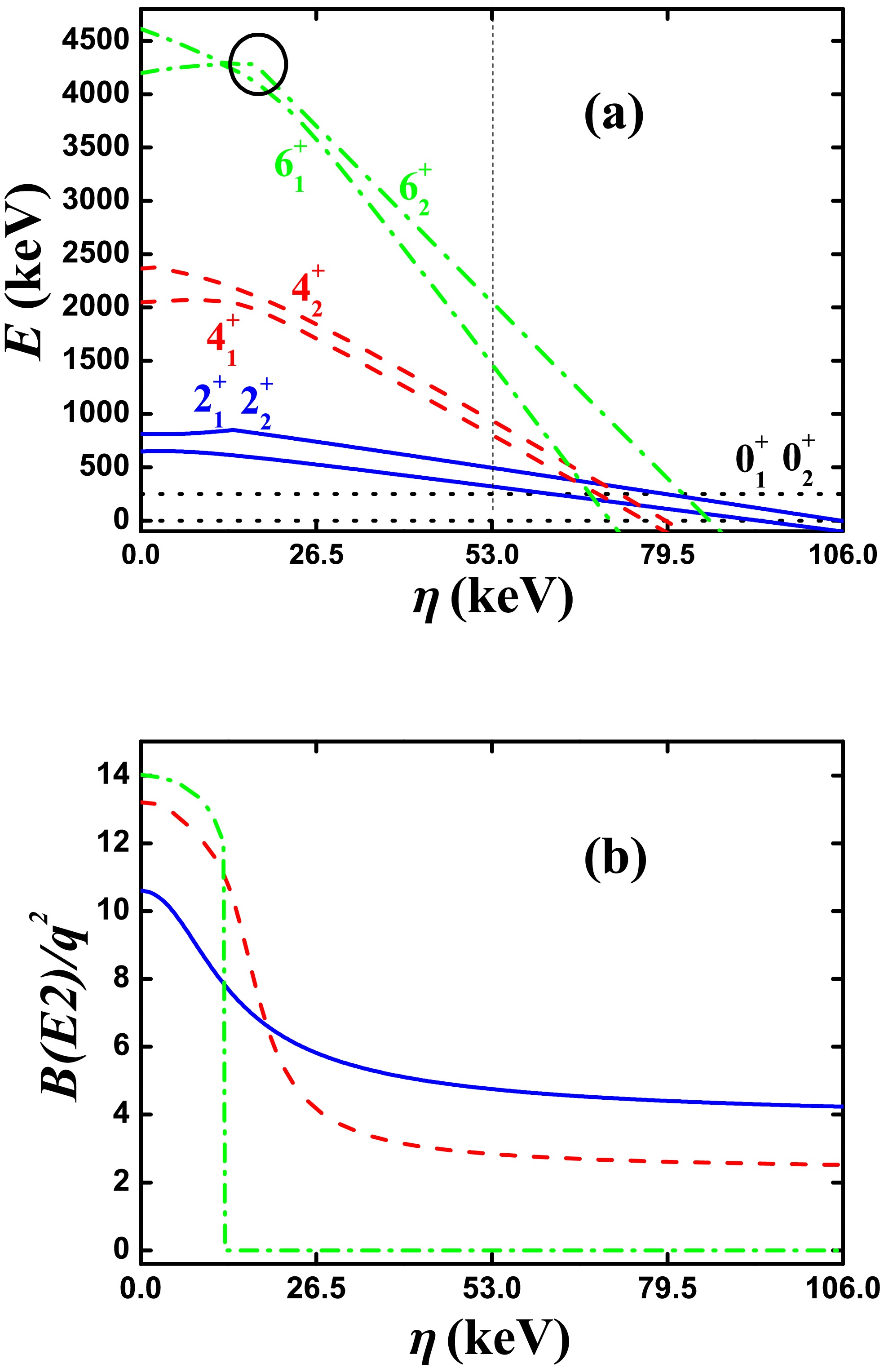

Figure 2.(color online) (a) Evolutional behaviors of the partial low-lying levels as functions ofη; (b) evolutional behaviors of $ B(E2; 2_{1}^{+}\rightarrow 0_{1}^{+}) $ (blue real line), $ B(E2; 4_{1}^{+}\rightarrow 2_{1}^{+}) $ (red dashed line), and $ B(E2; 6_{1}^{+}\rightarrow 4_{1}^{+}) $ (green dashed dotted line) as functions ofη. The parameters were deduced from Ref. [41].

In Ref. [41], another group of parameters for $ ^{168} {\rm{Os}}$ was reported: $ \alpha = 99 $ keV, $ \beta = 50.4 $ keV, $ \gamma = 3.5 $ keV, $ \delta = 0.55 $ keV, $ \eta = 43 $ keV, $ \zeta = -9.7 $ keV, and $ \xi = 26 $ keV. ForSU(3) analysis, let $ \alpha = 0 $ .Fig. 3(a) shows the evolutional behaviors of the partial low-lying levels as functions ofηfrom 0 to 86 keV, and the middle point is the parameter reported in Ref. [41] ( $ \eta = 43 $ keV). Clearly, the $ 4_{1}^{+} $ state intersects with one other $ 4^{+} $ state at $ \eta = 23 $ keV (red dashed lines) and the $ 6_{1}^{+} $ state intersects with one other $ 6^{+} $ state at $ \eta = 30.1 $ keV (green dashed dotted lines), which is larger than that of the $ 4^{+} $ states at the crossing point (two black circles). Thus, thisB(E2) anomaly results from level-crossing effects. However, these crossing effects may be complex. Thus, confirming real crossing effects in experimental results requires more experimental data. If this is the case, the emergence of theB(E2) anomaly may be an accidental effect. InFig. 3(b), the $ B(E2; 4_{1}^{+}\rightarrow 2_{1}^{+}) $ and $ B(E2; 6_{1}^{+}\rightarrow 4_{1}^{+}) $ anomalies occur simultaneously. TheSU(3) irrep. of the ground state is (2,4) ( $ \gamma = 35.8^{\circ} $ according to Eq. (7)); therefore, theB(E2) values become smaller, if they exist.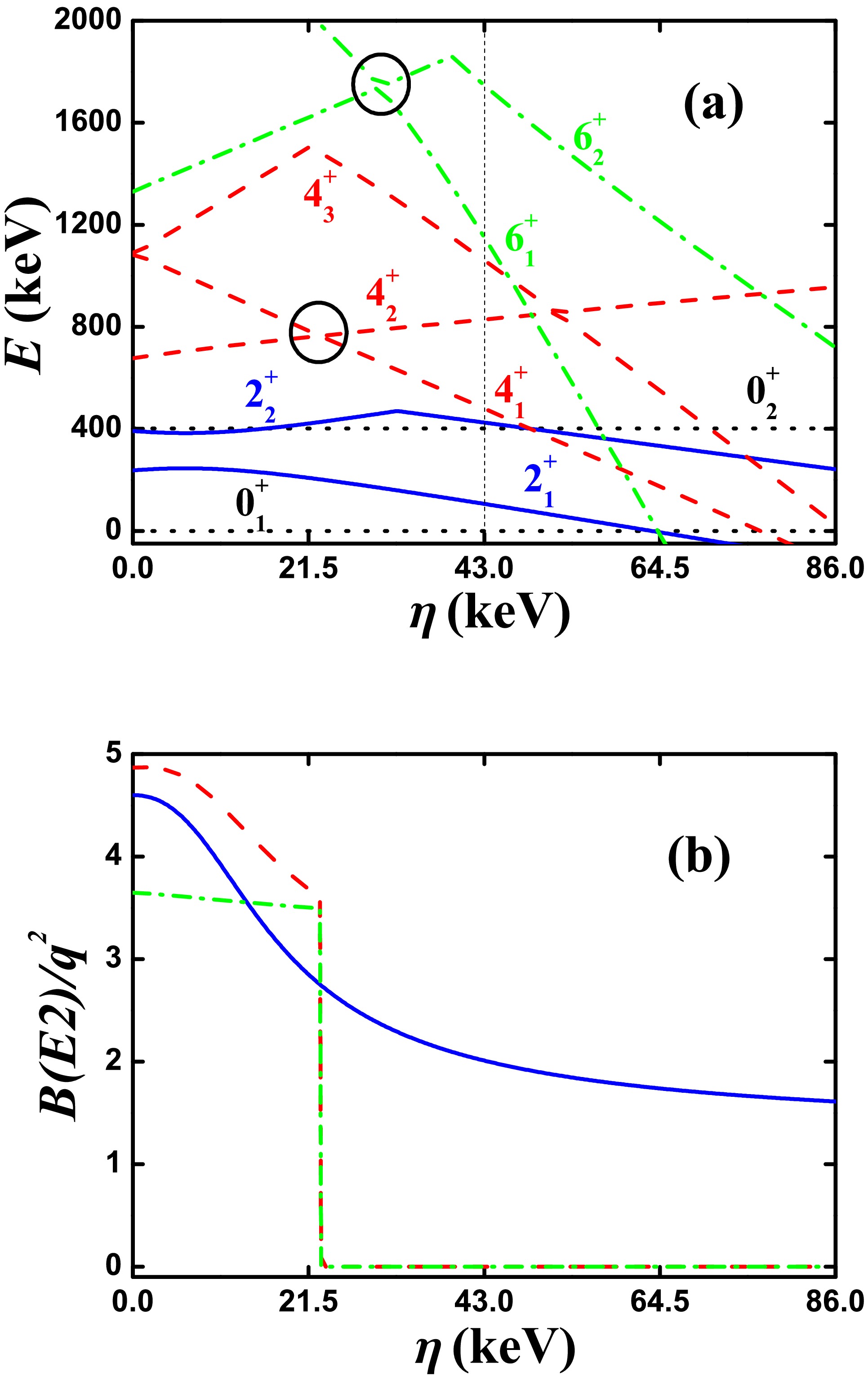

Figure 3.(color online) (a) Evolutional behaviors of the partial low-lying levels as functions ofη; (b) Evolutional behaviors of $ B(E2; 2_{1}^{+}\rightarrow 0_{1}^{+}) $ (blue real line), $ B(E2; 4_{1}^{+}\rightarrow 2_{1}^{+}) $ (red dashed line), and $ B(E2; 6_{1}^{+}\rightarrow 4_{1}^{+}) $ (green dashed dotted line) as functions ofη. The parameters were deduced from Ref. [41].

When analyzing theB(E2) anomaly, both the ratio $ B_{4/2} $ and absolute value of $ B(E2;2_{1}^{+}\rightarrow 0_{1}^{+}) $ should be considered. If the nuclei $ ^{172} {\rm{Pt}}$ , $ ^{168,170} {\rm{Os}}$ , and $ ^{166} {\rm{W}}$ with theB(E2) anomaly are put in the isotopic evolutions [19−22], the results vary continuously. This is also key for considering these spectra as collective excitations. Extremely small $ B(E2;2_{1}^{+}\rightarrow 0_{1}^{+}) $ values imply a large effective chargeq, which may not be reasonable (see Ref. [52]).

In previous IBM versions,O(5) symmetry exists when evolving from theU(5) toO(6) limits, which results in the crossover of the $ 0_{2}^{+} $ and $ 0_{3}^{+} $ states. When the parameters slightly deviate, significant energy level exclusion can occur [18]. This is important to confirm such phenomena. Recently, in the SU3-IBM, similar results were reported in Ref. [54]: it is a level-anticrossing phenomenon.

Important new results were reported recently. In Ref. [44], theSU(3) quadrupole operator $ \hat{Q} $ was replaced by the generalized quadrupole operator $ \hat{Q}_{\chi} $ . We also take $ ^{168} {\rm{Os}}$ as an example, setting $ \alpha = 0 $ , $ \beta = -25.0 $ keV, $ \gamma = 0 $ , $ \delta = 0 $ , $ \eta = -26.9 $ keV, $ \zeta = 0 $ , $ \xi = 43.65 $ keV, and $ \chi = -0.39 $ . ForSU(3) analysis, let $ \chi = -\frac{\sqrt{7}}{2} $ . Here, theSU(3) irrep. of the ground state is (16,0) with prolate shape.Fig. 4(a) shows the evolutional behaviors of the partial low-lying levels as functions ofηfrom 0 to −53.8 keV; the middle point is the parameter reported in Ref. [44] ( $ \eta = -26.9 $ keV). Intuitively, this evolutional behavior is similar to those inFig. 1(a). The $ 4_{1}^{+} $ state intersects with one other $ 4^{+} $ state at $ \eta = -44.8 $ keV (red dashed lines), and the $ 6_{1}^{+} $ state also intersects with one other $ 6^{+} $ state at $ \eta = -29.4 $ keV (green dashed dotted lines). The two crossover points are marked by black circles. This means that thisB(E2) anomaly is also related with theSU(3) symmetry.

Figure 4.(color online) (a) Evolutional behaviors of the partial low-lying levels as functions ofη; (b) evolutional behaviors of $ B(E2; 2_{1}^{+}\rightarrow 0_{1}^{+}) $ (blue real line), $ B(E2; 4_{1}^{+}\rightarrow 2_{1}^{+}) $ (red dashed line), and $ B(E2; 6_{1}^{+}\rightarrow 4_{1}^{+}) $ (green dashed dotted line) as functions ofη. The parameters were deduced from Ref. [44].

Note that the middle point shows a normal $ B_{4/2} $ value but is close to the anomalous region. This is interesting, revealing a new mechanism for theB(E2) anomaly related with the level-anticrossing phenomenon. This new mechanism was discussed in detail in Ref. [66]. It was found that theB(E2) anomaly in theSU(3) symmetry limit and theB(E2) anomaly along the transitional region from theSU(3) symmetry limit to theO(6) symmetry limit are closely related. These results can help further explain the anomalous small $ B(E2;2_{1}^{+}\rightarrow 0_{1}^{+}) $ value in $ ^{166} {\rm{Os}}$ [60].

A reasonable theory may be useful not only for explaining small $ B_{4/2} $ values but also for considering normal $ B(E2;2_{1}^{+}\rightarrow 0_{1}^{+}) $ values in $ ^{172} {\rm{Pt}}$ , $ ^{168,170} {\rm{Os}}$ , and $ ^{166} {\rm{W}}$ and for explaining the anomalous small $ B(E2;2_{1}^{+}\rightarrow 0_{1}^{+}) $ value in $ ^{166} {\rm{Os}}$ [59]. This is addressed in Ref. [60].

In Ref. [46] , a new mechanism at the oblate side was reported. We also take $ ^{168} {\rm{Os}}$ as an example, where $ \alpha = 72.0 $ keV, $ \beta = -7.825 $ keV, $ \gamma = 2.636 $ keV, $ \delta = 0 $ , $ \eta = 15.1 $ keV, $ \zeta = -1.09 $ keV, and $ \xi = 36.87 $ keV. ForSU(3) analysis, let $ \alpha = 0 $ . Here, theSU(3) irrep. of the ground state is (0,8) with the oblate shape.Fig. 5(a) shows the evolutional behaviors of the partial low-lying levels as functions ofηfrom 0 to 30.2 keV; the middle point is the parameter reported in Ref. [46] ( $ \eta = 15.1 $ keV). Note that the $ 2_{1}^{+} $ and $ 2_{2}^{+} $ states intersect with each other at $ \eta = 12.1 $ keV (blue real lines), the $ 4_{1}^{+} $ and $ 4_{2}^{+} $ states intersect with each other at $ \eta = 4.6 $ keV (red dashed lines), and the $ 6_{1}^{+} $ and $ 6_{2}^{+} $ states intersect with each other at $ \eta = 2.5 $ keV (green dashed dotted lines). The three crossover points are marked by black circles. At the middle point, the $ B_{4/2} $ value is infinity. This is interesting. We also confirm that thisB(E2) anomaly is related with theSU(3) symmetry. This new mechanism is discussed in Section V in detail.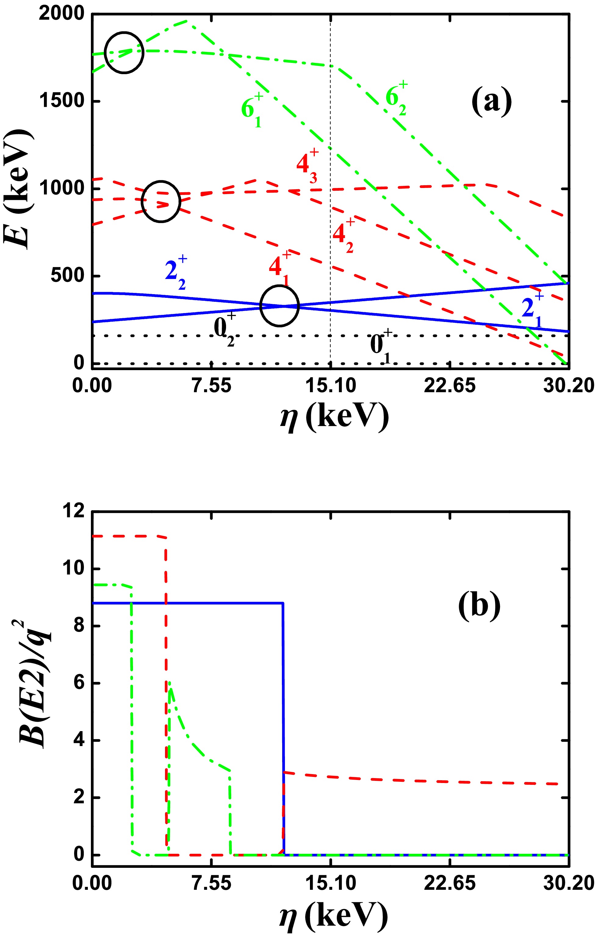

Figure 5.(color online) (a) Evolutional behaviors of the partial low-lying levels as functions ofη; (b) evolutional behaviors of $ B(E2; 2_{1}^{+}\rightarrow 0_{1}^{+}) $ (blue real line), $ B(E2; 4_{1}^{+}\rightarrow 2_{1}^{+}) $ (red dashed line), and $ B(E2; 6_{1}^{+}\rightarrow 4_{1}^{+}) $ (green dashed dotted line) as functions ofη. The parameters were deduced from Ref. [46].

The results in the aformentioned five examples broaden our understanding of theB(E2) anomaly. Even if the conditions that (1) the $ B(E2; 2_{1}^{+}\rightarrow 0_{1}^{+}) $ value exists and (2) $ B(E2; 4_{1}^{+}\rightarrow 2_{1}^{+}) $ is 0 are not satisfied in theSU(3) symmetry limit, theB(E2) anomaly may still appear.

If an explanation for theB(E2) anomaly can include aSU(3) symmetry limit,SU(3) analysis should be performed. From the above examples and Refs. [40−47], we provide a great deal of new results. There are some phenomena that seem to have nothing to do with theSU(3) symmetry but are actually related with it. This may be a more complicated mechanism that requires further elaboration (see Ref. [66]). InSU(3) analysis, if no level-crossing occurs but theB(E2) anomaly still appears, it can be attributed to the rigid triaxial rotor effect. The case in which noB(E2) anomaly exists in theSU(3) analysis but theB(E2) anomaly appears when thedboson number operator is added (which is almost impossible), or $ \hat{Q} $ is replaced by $ \hat{Q}_{\chi} $ , is critical. A general discussion will be provided with the extendedQ-consistent Hamiltonian including up to fourth-order interactions. In a previous study [38], it was demonstrated that, for this extended Hamiltonian, when $ \chi = 0 $ , that is, at theO(6) symmetry limit, theB(E2) anomaly cannot occur. Thus, it is important to discuss the evolving region from theSU(3) symmetry limit to theO(6) symmetry limit.

For the first and fourth examples, the values of the parameterηfor the fourth-order interactions $ [(\hat{L}\times \hat{Q})^{(1)} \times (\hat{L} \times \hat{Q})^{(1)}]^{(0)} $ are 0. Thus, the evolutional behaviors of theB(E2) values inFigs. 1(b) and4(b) are simple. When these interactions are added, more complex evolutional behaviors can be observed, which is interesting. Although these interactions were studied within the context of the rigid triaxial explanation [41,46,47,58], many details were inadequate. For the second and third examples, the sign ofηis negative, and the evolutional behaviors of theB(E2) values inFigs. 2(b) and3(b) become more complex (the evolution lines become curved). However, they are still similar to the cases inFigs. 1(b) and4(b). For the fifth example, the sign ofηis positive, and the evolutional behaviors of theB(E2) values inFig. 5(b) become more complex than those inFigs. 2(b) and3(b). Thus, further discussion on the $ [(\hat{L}\times \hat{Q})^{(1)} \times (\hat{L} \times \hat{Q})^{(1)}]^{(0)} $ interaction is necessary to understand the more complexB(E2) anomaly, for example in $ ^{72,74} {\rm{Zn}}$ [29−31] and $ ^{114} {\rm{Te}}$ [32,33].

In this section, we further discuss the new mechanism presented inFig. 5[46]. InFig. 5(b), the changes in the values of $ B(E2; 2_{1}^{+}\rightarrow 0_{1}^{+}) $ (blue real line), $ B(E2; 4_{1}^{+}\rightarrow 2_{1}^{+}) $ (red dashed line), and $ B(E2; 6_{1}^{+}\rightarrow 4_{1}^{+}) $ (green dashed dotted line) are similar to those inFig. 1(b) but exhibit more complicated behaviors. The key for these behaviors is the introduction of the fourth-order interaction $ [(\hat{L}\times \hat{Q})^{(1)} \times (\hat{L} \times \hat{Q})^{(1)}]^{(0)} $ . The effect of theSU(3) fourth-order interactions on theB(E2) anomaly is complex, and a detailed discussion will be addressed in the future. Here, just the parameters reported in Ref. [46] are considered. We can see that the fourth-order interaction brings in new features.

InFig. 5(b), when $ \eta = 15.1 $ keV (the parameter used was reported in Ref.[46]), $ B(E2; 2_{1}^{+}\rightarrow 0_{1}^{+}) = 0 $ while $ B(E2; 4_{1}^{+}\rightarrow 2_{1}^{+})\neq 0 $ . Thus, $ B_{4/2} = \infty $ , which is a new result. When $ \eta = 11.325 $ keV, $ B(E2; 2_{1}^{+}\rightarrow 0_{1}^{+})\neq0 $ while $ B(E2; 4_{1}^{+}\rightarrow 2_{1}^{+}) = 0 $ . Thus, $ B_{4/2} = 0 $ , which was reported in a previous study. For both cases, $ B(E2; 6_{1}^{+}\rightarrow 4_{1}^{+}) = 0 $ . When $ \eta = 7.55 $ keV, $ B(E2; 2_{1}^{+}\rightarrow 0_{1}^{+})\neq 0 $ , $ B(E2; 4_{1}^{+}\rightarrow 2_{1}^{+}) = 0 $ while $ B(E2; 6_{1}^{+}\rightarrow 4_{1}^{+})\neq 0 $ . When the fourth-order interaction is introduced, anyB(E2) results may be obtained.

The evolutional trends are similar.Figs. 6−8(b) show the evolutional behaviors of the values of $ B(E2; 2_{1}^{+}\rightarrow 0_{1}^{+}) $ , $ B(E2; 4_{1}^{+}\rightarrow 2_{1}^{+}) $ , and $ B(E2; 6_{1}^{+}\rightarrow 4_{1}^{+}) $ as functions ofαwhen $ \eta = 15.1 $ , 11.325, and 7.55 keV. The evolutional trends are notably different.

Figure 6.(color online) (a) Evolutional behaviors of the partial low-lying levels as functions ofα; (b) evolutional behaviors of $B(E2; 2_{1}^{+}\rightarrow 0_{1}^{+})$ (blue real line), $B(E2; 4_{1}^{+}\rightarrow 2_{1}^{+})$ (red dashed line), and $B(E2; 6_{1}^{+}\rightarrow 4_{1}^{+})$ (green dashed dotted line) as functions ofα. The parameters were deduced from Ref. [46] ( $\eta=15.1$ keV).

Figure 7.(color online) (a) Evolutional behaviors of the partial low-lying levels as functions ofα; (b) Evolutional behaviors of $B(E2; 2_{1}^{+}\rightarrow 0_{1}^{+})$ (blue real line), $B(E2; 4_{1}^{+}\rightarrow 2_{1}^{+})$ (red dashed line), and $B(E2; 6_{1}^{+}\rightarrow 4_{1}^{+})$ (green dashed dotted line) as functions ofα. The parameters were deduced from Ref. [46] but $\eta=11.325$ keV.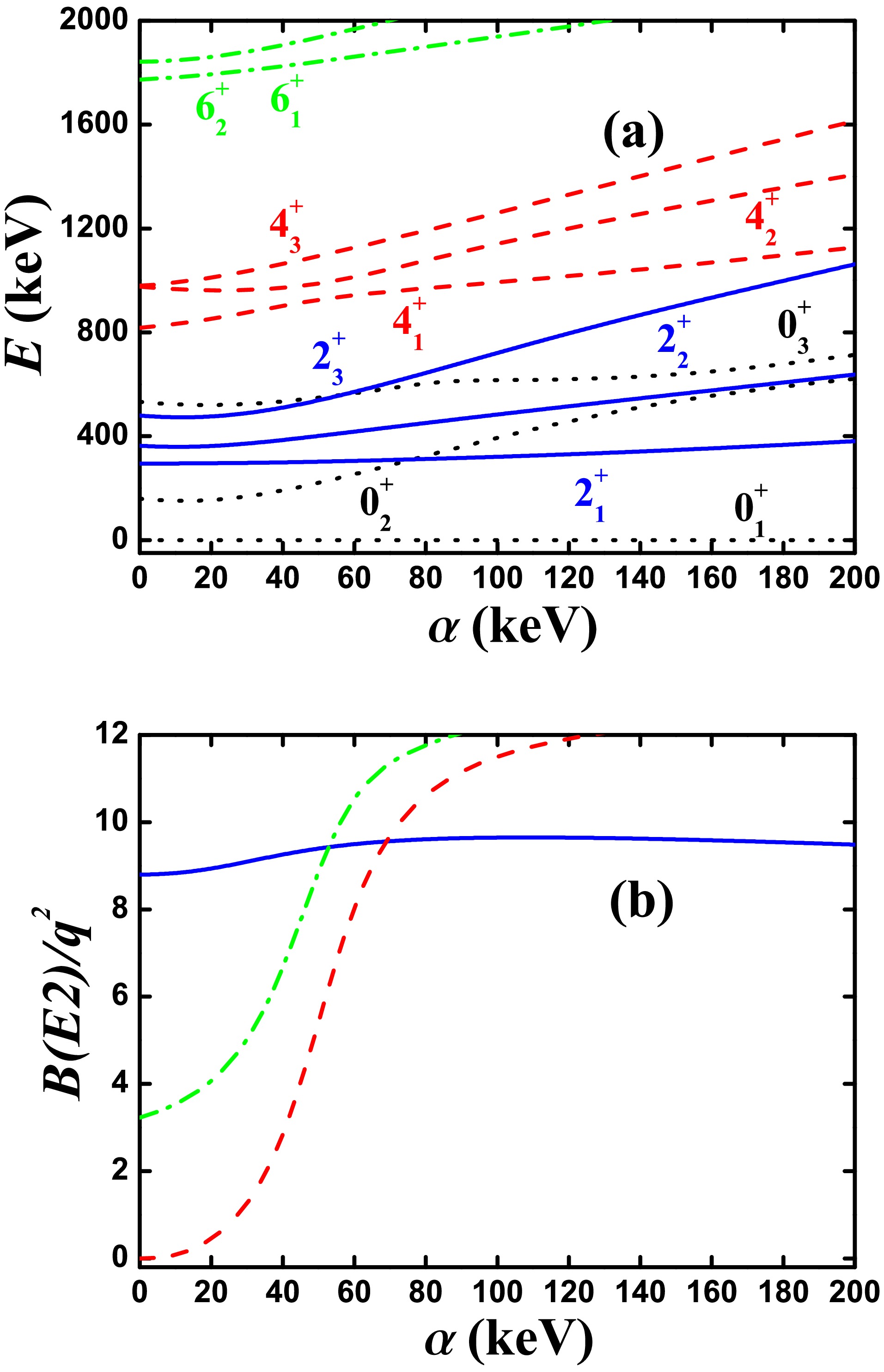

Figure 8.(a) Evolutional behaviors of the partial low-lying levels as functions ofα; (b) evolutional behaviors of $B(E2; 2_{1}^{+}\rightarrow 0_{1}^{+})$ (blue real line), $B(E2; 4_{1}^{+}\rightarrow 2_{1}^{+})$ (red dashed line), and $B(E2; 6_{1}^{+}\rightarrow 4_{1}^{+})$ (green dashed dotted line) as functions ofα. The parameters were deduced from Ref. [46] but $\eta=7.55$ keV.

Fig. 9presents the evolutional behaviors of the $ B_{4/2} $ values as functions ofαfor $ \eta = 15.1 $ keV, $ \eta = 11.325 $ keV, and $ \eta = 7.55 $ keV. Other parameters were deduced from Ref. [46]. In $ ^{168} {\rm{Os}}$ , $ B_{4/2} = 0.34 $ . For $ \eta = 15.1 $ keV, the smallest value is 0.45. In Ref. [46], $ B_{4/2} = 0.53 $ was used. In the following section, $ B_{4/2} = 0.45 $ is used for result 1 (black point). For $ \eta = 11.325 $ keV and 7.55 keV, $ B_{4/2} = 0.34 $ exists (blue and red points) and is used for results 2 and 3. For comparison, $ B_{4/2} = 0 $ is also used for result 4 when $ \eta = 7.55 $ keV, which is just the result ofSU(3) analysis on result 3.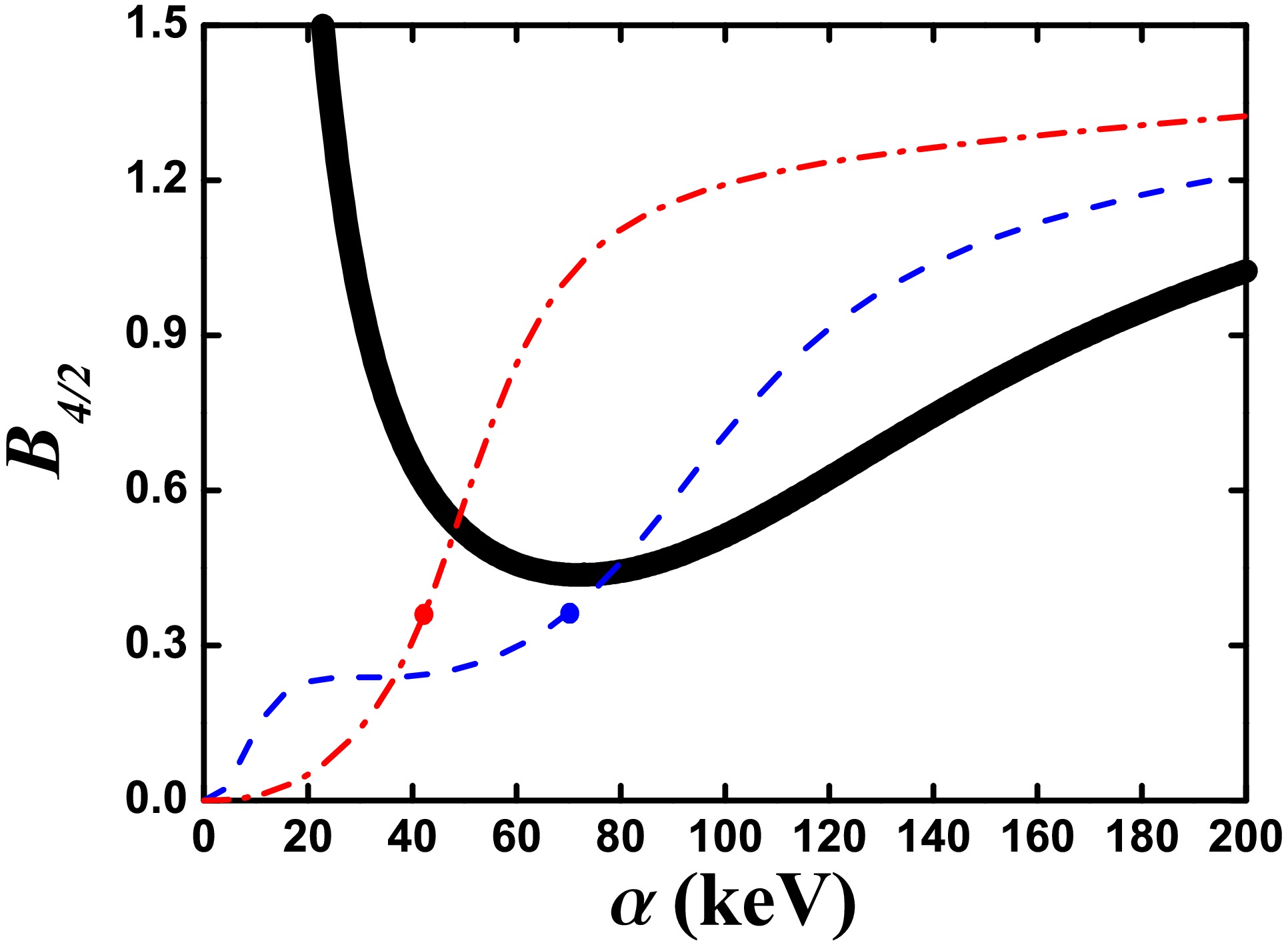

Figure 9.Evolutional behaviors of the $ B_{4/2} $ values as functions ofαfor $ \eta = 15.1 $ keV (black real line), $ \eta = 11.325 $ keV (blue dashed dotted line), and $ \eta = 7.55 $ keV (red dashed dotted line). Other parameters were deduced from Ref. [46].

If the fourth-order interaction $ [(\hat{L}\times \hat{Q})^{(1)} \times (\hat{L} \times \hat{Q})^{(1)}]^{(0)} $ is not added, theB(E2) values of each energy level in the yrast band can gradually decrease as the angular momentumLincreases [40,58]. However, when this interaction is added, this change becomes more irregular. This is important for understanding irregularB(E2) anomalies.

Results $ 1-3 $ correspond to the three points (black, blue, and red) inFig. 9. Result 4 corresponds to the $ \alpha = 0 $ point of the red line inFig. 9. Let the energy of the $ 2_{1}^{+} $ state be equal to the experimental one in $ ^{168} {\rm{Os}}$ . The parameters of the four results are shown inTable 1and the fitting values are listed inTable 2. For results 1, 2, and 3, the energies of the $ 0_{2}^{+} $ and $ 2_{2}^{+} $ states increase. For results 1 and 2, the values of $ B(E2; 8_{1}^{+}\rightarrow 6_{1}^{+}) $ are larger. For result 3, the value of $ B(E2; 6_{1}^{+}\rightarrow 4_{1}^{+}) $ is larger. Thus, theseB(E2) values are sensitive to the parameters. For result 4, the results of theSU(3) analysis are shown. The irregularity of theB(E2) values is clear whenLincreases. When $ \hat{n}_{d} $ is added, result 4 becomes result 3, which exhibits a better fitting effect. Level-crossing is indeed a possible reason for the emergence of theB(E2) anomaly. For a better understanding of theB(E2) anomaly in $ ^{168} {\rm{Os}}$ , more experimental results are needed.

	Exp.	Res. 1	Res. 2	Res. 3	Res. 4
$ E_{2_{1}^{+}} $	341	341	341	341	341
$ E_{4_{1}^{+}} $	857	857	857	867	857
$ E_{6_{1}^{+}} $	1499	1607	1586	1642	1898
$ E_{8_{1}^{+}} $	2223	2342	2136	2103	2771
$ E_{10_{1}^{+}} $	2983	3522	3248	2960	4213
$ E_{0_{2}^{+}} $		261	380	521	276
$ E_{2_{2}^{+}} $		424	463	575	461
$ E_{3_{1}^{+}} $		778	821	962	841
$ E_{4_{2}^{+}} $		1057	1055	1064	1130
$ B(E2;2^{+}_{1}\rightarrow 0^{+}_{1}) $	74(13)	74	74	74	74
$ B(E2;4^{+}_{1}\rightarrow 2^{+}_{1}) $	25(13)	33	25	25	0
$ B(E2;6^{+}_{1}\rightarrow 4^{+}_{1}) $		16	16	50	27
$ B(E2;8^{+}_{1}\rightarrow 6^{+}_{1}) $		57	49	11	0
$ B(E2;10^{+}_{1}\rightarrow 8^{+}_{1}) $		2.8	2.8	22	14

Table 2.Experimental and fitting values of the four results for $ ^{168} $ Os. The unit of the energy level is keV whereas that of theB(E2) value is W.u.. The effective charges of results 1-4 are 3.114 $ \sqrt{ \rm{W.u.}} $ , 2.2825 $ \sqrt{ \rm{W.u.}} $ , 2.823 $ \sqrt{ \rm{W.u.}} $ , and 2.900 $ \sqrt{ \rm{W.u.}} $ , respectively.

In this study, we proposed a powerful technique for understanding theB(E2) anomaly, namely theSU(3) analysis. By analyzing the examples in Refs. [40−47], new results were obtained. Three of these results are particularly relevant. First, theSU(3) third-order interaction $ [L\times Q \times L]^{(0)} $ is critical for theSU(3) anomaly. Whether this relationship is unique requires further investigation. Second, when this interaction is added, various level-crossing phenomena can occur. The causes of theB(E2) anomaly in realistic experiments require more experimental research. Searching for additional mechanisms for theB(E2) anomaly also seems necessary. Third, not only the value of $ B(E2;4_{1}^{+}\rightarrow 2_{1}^{+}) $ but also those of $ B(E2;6_{1}^{+}\rightarrow 4_{1}^{+}) $ and $ B(E2;2_{1}^{+}\rightarrow 0_{1}^{+}) $ can be anomalous. TheB(E2) anomaly in $ ^{168} {\rm{Os}}$ was discussed. It is critical to obtain more experimentalB(E2) anomaly results.