Supersymmetric hybrid inflation in light of CMB experiments and swampland conjectures

In the current era of TeV-scale physics, we have only discovered the Higgs boson at the Large Hadron Collider (LHC) [1,2], which completes the standard model of particle physics. We have experimental and theoretical reasons to believe that there exists physics beyond the standard model (BSM). Despite the intensive searches for BSM at the LHC [3−6], we have not found any evidence of it. Human curiosity is not restricted to terrestrial experiments, there are satellite-based experiments such as WMAP [7] and Planck [8], which can provide insights on the beginning of our universe. In most of the BSM scenarios, we need particles besides those in the SM to explain some of the mysteries of our universe. Supersymmetry (SUSY) is one of the most promising extension of the SM. The minimal SUSY version of the SM, that is, MSSM, provides the grand unification, that is, the gauge coupling unification, of the electromagnetic, weak, and strong interactions for solving the gauge hierarchy problem and depicting the dark matter particle. The grand unification is a holy grail of particle physics and, since its inception, has been waiting for experimental verification such as in proton decay experiments [9]. It is believed that the cosmic inflation took place near or at the grand unification scale $M_{\rm GUT}$ . Cosmic inflationary models naturally require input from particle physics, and those based on SUSY frameworks are particularly attractive. Specifically, models based on SUSY grand unified theories (SUSY GUTs) provide alternative grounds to look for BSM. SUSY hybrid inflationary models [10−13] are highly attractive because they naturally connect [14,15] low-scale ( $ \sim $ TeV) SUSY and minimal ( $ N=1 $ ) supergravity (SUGRA) [16−18].

The potential along the inflationary path at the tree level is flat in the simplest SUSY hybrid inflationary models. The radiative corrections (RC), when added to the scalar potential, produce the required slope of the inflationary track toward the SUSY vacuum, and in this process, gauge symmetry groupGbreaks to its subgroupHduring inflation [19] or at the end of inflation [10,11]. In such a scenario [10], the temperature anisotropy $ \delta T/T $ of the cosmic microwave background (CMB) turns out to be on the order of $ (M/m_P)^2 $ , whereMis the symmetry breaking scale ofG, and $ m_P $ is the reduced Planck mass. Then, in order to maintain the self-consistency of the inflationary scenario,Mis comparable to the scale of grand unification, $ M_{\rm GUT} \sim 10^{16} $ GeV, hinting thatGmay constitute a grand unified theory (GUT) group.

In SUSY hybrid inflation, it is important to note that the scalar spectral index $ n_{\rm s} $ falls within the observed range of 0.96−0.97, as indicated in [20]. This alignment is achievable when the inflationary potential incorporates radiative corrections [10] along with either the inclusion of soft SUSY breaking terms [21−25] or higher-order terms in the Kähler potential [26]. Conversely, if such terms are not included, $ n_{\rm s} $ lies close to 0.98. Such a value of $ n_{s} $ is only acceptable if the effective number of light neutrino species is slightly higher than 3 [20]. Given that approximately 50e-folds are required to resolve the horizon and flatness problem, the inflaton field values remain well below the Planck scale $ M_{P} $ ; thus, in both cases, the supergravity corrections remain under control.

In this article, we address two primary issues. The Planck collaboration [8] and LiteBIRD [27] have highlighted models that hold promise for observation in future experiments. In Fig. 8 of Ref. [8] and Fig. 2 and Fig. 3 of Ref. [27], it is asserted that the CMB depictions from [10] appear to have been ruled out. We address this problem in two ways. First, we employ the minimal Kähler potential, and taking into account radiative corrections and soft SUSY contributions along with SUGRA corrections, we show that SUSY hybrid inflation is consistent with Planck 2018 data [8] but faces one problem. Specifically, the gauge symmetry breaking scale in these scenarios becomes $ {\cal O}(10^{15}) $ GeV; this can lead to rapid proton decay through dimension-6 or dimension-5 operators, which are suppressed byM[28−36]. This problem can be avoided ifMis $ {\cal O}(10^{16}) $ GeV.

We display a parameter space where we not only have $ n_{s} $ consistent with Planck 2018 data but also achieveMon the order of $ 10^{16} $ GeV and thus avoid the proton decay rate problem. In these calculations, we use $ {\cal N}= $ 1 and $ {\cal N}= $ 2 ¹ , with the number ofe-folding $ N_{0} $ =50, and show that we can achieve this task with $ M_{S}^{2}< $ 0 and $ am_{3/2}> $ 0. Here, we have $ m_{3/2}\neq|M_{S}| $ and $ m_{3/2}= $ 1, 10, 100, and 1000 TeV. This comes at the cost of having the soft SUSY breaking scale $ |M_{S}|\gtrsim 10^{6} $ GeV and scalar to tensor ratiorbeing very small (between $ 10^{-15} $ to $ 10^{-8} $ ). In this scenario, since $ M_{S}^{2}< $ 0 and values ofrare very small, we also employ the non-minimal Kähler potential. In this case, we chose $ M=2\times 10^{16} $ GeV, $ N_{0}= $ 50, and $ M_{S}=am_{3/2}= $ 1 TeV with $ a=-1 $ along with $ \kappa_{S}< $ 0. We show that, in this case,rcan be in the range of $ 3\times 10^{-5} $ to $ 0.01 $ , while $ |S_{0}|/m_{p} $ is in the range of $ 0.02 $ to $ 1 $ .

The second issue we address in this article concerns the proposed swampland conjectures [37−40], which are discussed in detail later. It is hypothesized that cosmic inflation occurs at or near $ M_{\rm GUT} $ , describable by low-energy effective field theories (EFTs) [41−44]. These EFTs are reliable only if successfully embedded in a quantum theory of gravity, such as string theory. EFTs with UV completion are part of the landscape, while others, termed swampland theories, are inconsistent with quantum gravity when coupled to gravity [45,46]. For an extensive review, see [45,46]. The proposed swampland criteria originate from the weak gravity conjecture [47] and advancements in string theory and black hole physics [48]. These criteria serve as consistency checks on EFTs to determine if they belong to the swampland or the landscape. We also briefly discuss the swampland criteria and the Trans-Planckian censorship conjecture (TCC) [49,50] in the context of hybrid inflationary models.

The rest of the paper is organized as follows. In Sec. II, we provide details on the SUSY hybrid inflation model with minimal Kähler potential. In Sec. III, we describe the swampland conjecture and its variations. We present our numerical calculations for SUSY hybrid inflation with minimal and non-minimal Kähler potentials in Sec. IV. Finally, we summarize our results in Sec. V.

SUSY hybrid inflation models are described by the following normalizable superpotential [10,11]:

whereSis a gauge singlet superfield representing the inflaton, Φ and $ \overline{\Phi } $ are conjugate superfields that transform nontrivially under some gauge groupGand provide the vacuum energy associated with inflation,κis a dimensionless coupling constant, andMis the mass parameter corresponding to the scale at which gauge groupGis broken. The superpotential given in Eq. (1) possesses the gauge symmetryGalong with an additional $ U(1) $ R-symmetry, which is usually employed to suppress proton decay if $ Z_{2} $ is its subgroup. Also, $ U(1) $ R-symmetry provides a unique structure of superpotential, linear in S. Under the $ U(1)_R $ symmetry, the superpotentialWtransforms as $W \rightarrow {\rm e}^{{\rm i}\alpha}W$ , whereαis the $ U(1)_R $ charge. The chiral superfieldStransforms as $S \rightarrow {\rm e}^{i\alpha}S$ , and the fields Φ and $ \bar{\Phi}$ are neutral under this symmetry, transforming as $ \Phi \bar{\Phi} \rightarrow \Phi \bar{\Phi}$ . These transformation properties ensure that the superpotentialWis consistent with both $ U(1)_R $ symmetry and gauge symmetryG. The global SUSY F-terms are given by

where $ z_{i}\in \{\phi , \overline{\phi }, s\} $ represents the bosonic components of the superfields $ \Phi, \overline{\Phi },S $ , respectively. Using Eqs. (1)–(2), the tree level global SUSY potential in the D-flat direction, $ |\phi|=|\overline{\phi}| $ , is

Inflation begins along the local minimum at $ |\phi| = 0 $ (the inflationary track), commencing from a large $ |s| $ . An instability emerges at the waterfall point, denoted as $ |s_c|^2 = M^2 $ , where $ s_c $ is the value of $ |s| $ at which $ \dfrac{\partial^2V}{\partial s^2}\big|_s=0 $ . At this point, the field naturally transitions into one of the two global minima at $ |\phi|^2=M^2 $ , coinciding with the breaking of the gauge group G. The scalar potential is approximately quadratic in $ |\phi| $ at large $ |s| $ , while at $ |s|=0 $ , Eq. (3) transforms into a Higgs potential.

Along the inflationary track, the gauge groupGis unbroken. However, only the constant term $ V_0=\kappa^2 M^4 $ is present at the tree level, implying SUSY breaking during inflation. SUSY breaking splits the fermionic and bosonic mass multiplets, contributing to radiative corrections. The minimal (canonical) Kähler potential can be written as

The SUGRA scalar potential is given by

where $ z _{i}\in \{\phi , \overline{\phi }, s,\cdots\} $ represents the bosonic components of the superfields; here, we also define

$ D_{z_{i}^{*}}W^{*}=\left( D_{z_{i}}W\right) ^{*} $ , and $ m_{P}=M_P/\sqrt{8\pi} \simeq 2.4\times 10^{18} $ GeV is the reduced Planck mass. By including various terms such as those representing leading order SUGRA correction, radiative correction, and soft SUSY breaking, we may write the scalar potential along the inflationary trajectory (i.e. $ |\phi|=|\overline{\phi}|=0 $ ) as

Here,

represents radiative corrections, and

Here, the inflaton fieldsis defined as $ x \equiv |s|/M $ , whereMis a characteristic mass scale. The dimensionality of the representation of the conjugate pair of fieldsϕand $ \overline{\phi} $ under the gauge groupGis denoted by $ {\cal{N}} $ . The gravitino mass is represented by $ m_{3/2} $ , andQdenotes the renormalization scale. Additionally,Ais the complex coefficient associated with the trilinear soft-SUSY-breaking terms. Both the linear term with coefficientaand the mass-squared term $ M_S^2 $ in Eq. (7) arise from a gravity-mediated SUSY-breaking mechanism. It is important to note that the imaginary component ofSis neglected in this analysis, as previously described in [23].

In this study, we employ $ G\equiv U(1) $ , which may be identified as $ U(1)_{B-L} $ corresponding to $ {\cal N} $ =1, and the left-right symmetric model $G\equiv S U(3)_{C}\times S U(2)_{L}\times S U(2)_{R}\times U(1)_{B-L}$ corresponds to $ {\cal N}= $ 2. In Eq. (7), the last two terms correspond to soft SUSY-breaking linear and mass-squared terms, respectively, and can be derived from a gravity mediated SUSY breaking scheme [13].Using the standard slow-roll approximation, various inflationary parameters can be estimated as follows:

Additionally, in the slow-roll approximation, the scalar spectral index $ n_s $ , the tensor-to-scalar ratior, and the running of the scalar spectral index ${\rm d}n_s / {\rm d} \ln k$ can be determined.

The Planck constraint on the scalar spectral index $ n_{s} $ in the ΛCDM model for very small values ofrand $\dfrac{{\rm d} n_s}{{\rm d}\ln k}$ is [8]

The amplitude of the primordial spectrum is given by

which been measured by Planck to be $ A_{s}= 2.137 \times 10^{-9} $ at $ k_0 = 0.05\, \text{Mpc}^{-1} $ [20]. The last $ N_0 $ number ofe-folds before the end of inflation is

where $ x_e $ is the value of the field at the end of inflation, and $ x_0 $ is the value of the field at the pivot scale $ k_0 $ . The value of $ x_e $ is constrained either by the breakdown of the slow roll approximation or by a "waterfall" destabilization event taking place at the critical value $ x_c = 1 $ , if the slow roll approximation holds.

It is hypothesized that cosmic inflation occurs near the scale of $ M_{\rm GUT} $ and can be described using low-energy effective field theories (EFTs) [41−44]. If these EFTs are relevant to the potential theories that explain the observed universe, they may be successfully integrated into a quantum theory of gravity, such as string theory. EFTs that can be embedded within a UV-complete theory are considered part of the landscape, while those that cannot are classified as part of the swampland. When EFTs in the swampland are coupled with gravity, they render quantum gravity inconsistent. Advancements in quantum gravity and related fields [48] have led to the proposal of two swampland criteria, which serve as consistency checks to ensure that an EFT lies within the landscape. The swampland conditions relevant to inflation are outlined as follows [37,38]:

•Distance Conjecture. This conjecture imposes a limit on the excursion of scalar fields in reduced Planck units $ (m_p=\sqrt{\hbar c/8\pi G}=1) $ such that

Whenever $ \Delta \phi $ exceeds 1, an infinite tower of states becomes exponentially light, causing the effective field theory description to break down [37].

•Refined de Sitter Conjecture. Initially proposed in [38], the de Sitter Conjecture forbids both de Sitter maxima and minima. However, due to various counterexamples to de Sitter maxima, a refined version has been suggested, which permits maxima but continues to forbid de Sitter minima [39],

wherecand $ c' $ are constants of $ {\cal{O}}(1) $ . These relations are combined into one in [40]:

By defining $ c\equiv V'/V $ and $ c'\equiv-V''/V $ , this can be rewritten as

•Trans-Planckian Censorship Conjecture (TCC). Proposed by Bedroya and Vafa, the TCC posits that any inflationary model that stretches modes from sub-Planckian to super-Hubble scales must lie in the swampland [44,49,50]. This conjecture has significant implications for inflationary cosmology, particularly in constraining the total number ofe-folds $ N_{0} $ during inflation, which in turn, imposes upper limits on the inflationary scaleHand the tensor-to-scalar ratior.

These developments have led to numerous studies investigating the impact of swampland conditions on inflationary models [36]. These conjectures have significantly restricted inflationary models in four-dimensional spacetime. Following the conjectures of Vafaet al., many physicists have explored swampland conditions, especially those related to de Sitter conjectures due to their experimental contradictions. Dvaliet al. [48] interpreted the de Sitter condition in terms of quantum breaking as follows:

•Bound on Extrema. The classical break-time $ t_{CL} $ is defined as the timescale after which classical nonlinearities dominate the system's evolution. Conversely, the quantum break-time $ t_Q $ is the timescale after which the system can no longer be described classically, regardless of how well classical nonlinearities are accounted for. Dvaliet al. [48] showed that, for a system with interaction strengthκ, the quantum break-time is given by $ t_Q = t_{CL}/\kappa $ . To avoid quantum de Sitter break-time, the following bound must be satisfied:

Given that the slow-roll parameter $ \eta \equiv \dfrac{V''}{V} \ll 1 $ , this quantum breaking-bound is equivalent toη.

•Bound on Slow-Roll. In the slow-roll regime, the potential $ V(\phi) $ is away from extrema. Due to the quantum breaking bound, the change in potential $ \Delta V $ over some time $ \Delta t \sim t_Q $ must satisfy $ |\Delta V| \gtrsim V $ . Approximating $ \Delta V \sim V' \dot{\phi} \Delta t $ and assuming the slow-roll condition $ \dot{\phi} \sim -V'/H $ , we get $ \Delta V \sim -V'^2 \Delta t / H $ . Considering $ t_{CL} \sim H^{-1} $ in the slow-roll case, we obtain

where $ \alpha = N_{sp} H^2 $ is the effective strength of graviton scattering for characteristic momentum transferH, and $ N_{sp} $ is the number of light particle species [51]. Another slow-roll parameter $ \epsilon $ can be expressed as $ \sqrt{2\epsilon} \equiv \dfrac{|V^\prime|}{V} $ , implying $ \sqrt{2\epsilon} \gtrsim \sqrt{\alpha} $ .

In this section, using slow roll equations (Eq. (10)), we perform a series of numerical calculations to analyze the implications of the model and discuss its predictions regarding the various cosmological observables. Our numerical analysis focuses on six independent key parameters:κ,M, $a m_{3/2}$ , $M_S^2$ , $x_0$ , and $x_e$ . These parameters are constrained by the following essential conditions:

• The amplitude of the scalar power spectrum, $A_s(k_0)$ , which has a fixed value of $2.137 \times 10^{-9}$ at $ k_0 = 0.05\, \text{Mpc}^{-1} $ [20].

• The scalar spectral index, $n_s$ , set to a fixed value of 0.9665 [20].

• The end of inflation, determined by the waterfall mechanism, with the condition $x_e = 1$ .

• The number ofe-folds, $N_0$ , which is fixed as 50.

These constraints are critical and play a key role in determining the possible outcomes predicted by the model. We divide our analysis into two cases: minimal Kähler and non-minimal Kähler potential. We show that the SUSY hybrid inflation model with a minimal Kähler potential remains consistent with Planck 2018 data without introducing a proton decay problem and satisfies the modified swampland conjectures. However, satisfying the TCC is difficult in the minimal case. To address the largersolutions and TCC, we consider Hybrid inflation with non-minimal Kähler potential. With non-minimal Kähler potential, we have largeras well as very smallr, which is required to satisfy the swampland conjecture and TCC. The details of numerical results are presented in the following subsections.

InFig. 1,we present plots in the $ r-n_{s} $ plane. In the left plot, we only include the first two terms of the scalar potential in Eq. (7), comprising SUGRA and radiative corrections. The plot in the right panel also includes a contribution of soft SUSY breaking terms. In these plots, we set the number ofe-folding $ {N_{0}} $ =50 and $ N_{0} $ =60 , while keeping $ M_{S}=am_{3/2} $ = 1 TeV with a negative sign fora. The horizontal light blue (dark blue) band displays the 1σ(2σ) variation from the central values of $ n_{s} $ =0.9665 [8]. From the left panel, it is evident that, without adding contributions of soft SUSY breaking terms to the scalar potential, the hybrid-inflation model is ruled out according to Planck 2018 data. In contrast, from the plot in the right panel, we see that, if we also include contributions of soft SUSY breaking terms to the scalar potential, the hybrid-inflationary model is still consistent with [8]. In these plots, we also notice that, for $ n_{s} $ to remain within 2 σ variation,rshould be less than $ 10^{-12} $ . At minimalWandK, we divide our analysis in two cases, $ M^{2}_{S}>0 $ and $ M^{2}_{S}<0 $ , which we discuss briefly as follows.

Figure 1.(color online) Plots for $ n_{s} $ vs.rfor $ {N_{0}}= $ 50 (blue curve) and $ {N_{0}} $ =60 (curve). The vertical light blue (dark blue) band shows the 1σ(2σ) variation from the central value of $ n_s = 0.9665 $ . The left panel shows that, without the contributions of soft SUSY breaking terms to the scalar potential, the hybrid inflation model is ruled out by Planck 2018 observations [8]. In contrast, the right panel demonstrates that, when the contributions of soft SUSY breaking terms are included in the scalar potential, the hybrid inflation model remains consistent with the Planck 2018 constraints.

InFig. 2, we show plots of $ \kappa-n_{s} $ and $ M-n_{s} $ planes at $ M_{S}=am_{3/2} $ = 1 TeV, with the sign ofabeing negative for $ {\cal{N}} $ =1 (blue curve) and $ {\cal{N}} $ =2 (purple curve). The horizontal blue bands have the same color coding as inFig. 1. From the left panel, we observe that, for maintaining consistency with Planck 2018 data, we require $ 10^{-4}\lesssim \kappa \lesssim 10^{-3} $ for both $ {\cal{N}} $ =1 and $ {\cal{N}} $ =2. The plot in the right panel reveals that, in this scenario, the gauge symmetry breaking scaleMis in the range $ \sim 1 \times 10^{15} $ to $ 1.5\times 10^{15} $ GeV. This relatively small value ofMcan cause a proton-decay problem, despite our results being consistent with Planck 2018 data [8].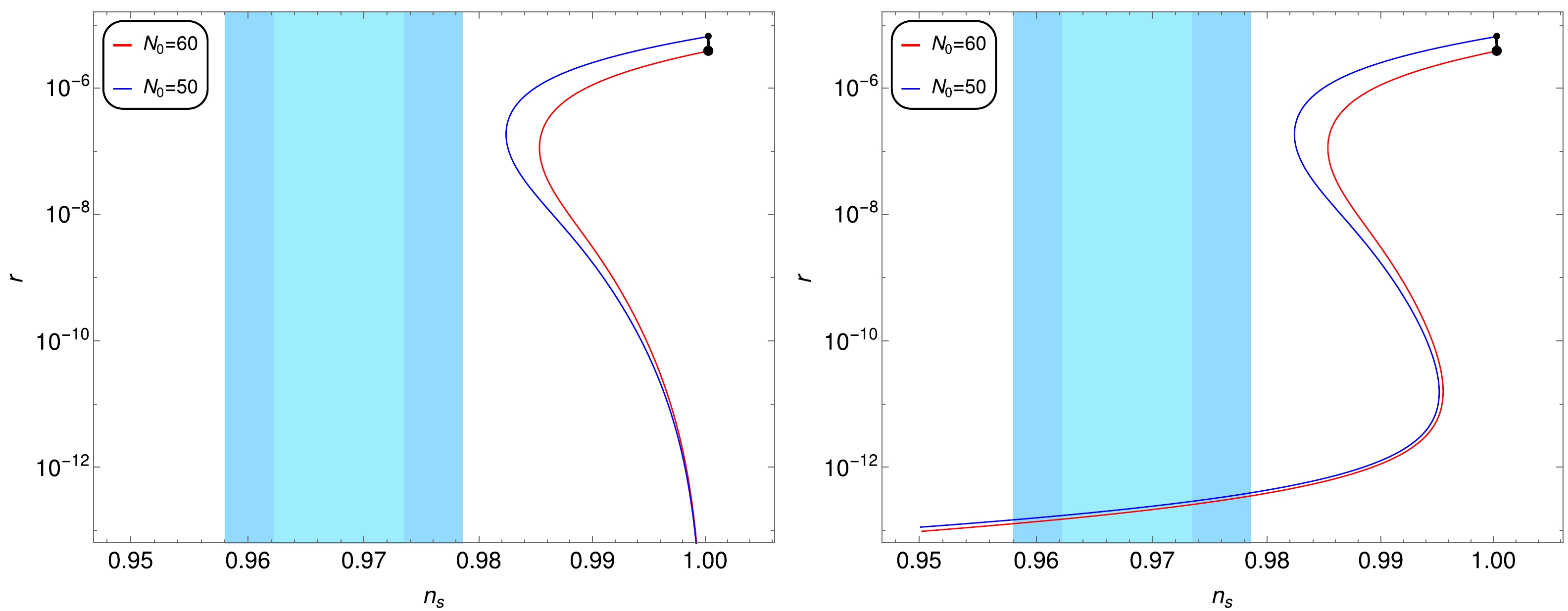

Figure 2.(color online) Plots for $ n_{s} $ vs.κandMv.sκfor $ {\cal{N}}=1 $ (blue curves) and $ {\cal{N}}=2 $ (purple curves). The horizontal light blue (dark blue) bands represent the 1σ(2σ) variation from central value of $ n_s = 0.9665 $ [8].

In this subsection, we briefly discuss how one can overcome the problem of smallness ofMat minimal Khäler potential while satisfying current Planck bounds [8] on $ n_{s} $ . InFig. 3andFig. 4we keep $ n_{s}= $ 0.9665 (central value) [8] and $ N_{0}= $ 50, with $ m_{3/2} \neq M_{S} $ . Notably, the gauge symmetry breaking scale turns out to be $ {\cal O}(10^{15}) $ GeV with $ M_{S}^2 > $ 0 [52]. This leaves us with $ M_{S}^{2}< $ 0. Now, $ am_{3/2} $ can be $ am_{3/2}= $ 0, $ am_{3/2}< $ 0, or $ am_{3/2}> $ 0. With $ M_{S}^{2}< $ 0 and $ am_{3/2}= $ 0,Magain turns out be $ {\cal O}(10^{15}) $ or less [53]. Thus, we have two cases, that is, $ M_{S}^{2}< $ 0 with $ am_{3/2}> $ 0 or $ am_{3/2}< $ 0. The second case is also discussed in [52]. With these two combinations, we plot for $ {\cal{N}} $ =1 and $ {\cal N} $ =2 with $ m_{3/2} $ = 1, 10, 100, and 1000 TeV. For $ {\cal N} $ =1 , the red curves represent $ am_{3/2}> $ 0 and blue curves represent $ am_{3/2}< $ 0, while the green curves represent $ am_{3/2}> $ 0 and purple curves represent $ am_{3/2}< $ 0 for $ {\cal N}= $ 2. Plots of the $ r-M $ plane are shown in the upper panel, while the lower panel shows plots of the $ |M_{S}|-M $ plane. From the top panel, it is evident that, for $ am_{3/2}< $ 0, that is, blue curves and purple curves, $ M\sim 10^{15} $ GeV , which is not acceptable due to the proton decay problem, which requires $ M\sim 10^{16} $ GeV. In contrast, in the case of $ M_{S}^{2}<0 $ and $ am_{3/2}> $ 0, that is, red and green curves, we have $ M\sim 10^{16} $ GeV for $ m_{3/2} $ = 1, 10, 100, and 1000 TeV. We also notice that the small value of tensor to scalar ratioris in the range of $ 10^{-15} $ to $ 10^{-8} $ (red and green curves). The lower panel gives us ranges of the gauge symmetry breaking scaleMand Soft SUSY breaking mass of singlet $ |M_{S}| $ . We note that, for $ |M_{S}|<10^{7} $ GeV with $ am_{3/2}< $ 0,Mis not sensitive to the values of $ |M_{S}| $ . As $ |M_{S}| $ keeps increasing up to $ 10^{10} $ GeV,Malso increases, approaches a maximum value ( $ M\sim 4\times 10^{15} $ GeV for $ m_{3/2}= $ 1000 TeV), and then starts to decrease. Conversely, some cancellation takes place when $ M_{S}^{2}<0 $ and $ am_{3/2}> $ 0. Consequently,Mstarts rising for $ |M_{S}|\gtrsim 10^{6} $ GeV. This shows that, in SUSY hybrid inflation, we can achieveMon the order of $ {10^{16}} $ GeV at a higher Soft SUSY breaking mass of singlet $ |M_{S}|\gtrsim 10^{6} $ GeV for both $ {\cal N} $ =1 and $ {\cal N} $ =2 with $ m_{3/2} $ = 1, 10, 100, and 1000 TeV. These large values of soft masses correspond to the Split-SUSY scenario [54,55].

Figure 3.(color online) Plots of $ r-M $ (upper panels) and $ |M_{S}|-M $ (lower panel) for $ N_0 = $ 50, $ n_s = 0.9665 $ (central value) [8], and $ M_{S}^{2}<0 $ . Curves for $ am_{3/2} > $ 0 (color) and $ am_{3/2} < $ 0 (blue color) at $ {\cal{N}} $ =1 and curves for $ am_{3/2} > $ 0 (green color) and $ am_{3/2} < $ 0 (purple color) at $ {\cal{N}} $ =2 and $ m_{3/2} $ =1, 10, 100 and 1000 TeV.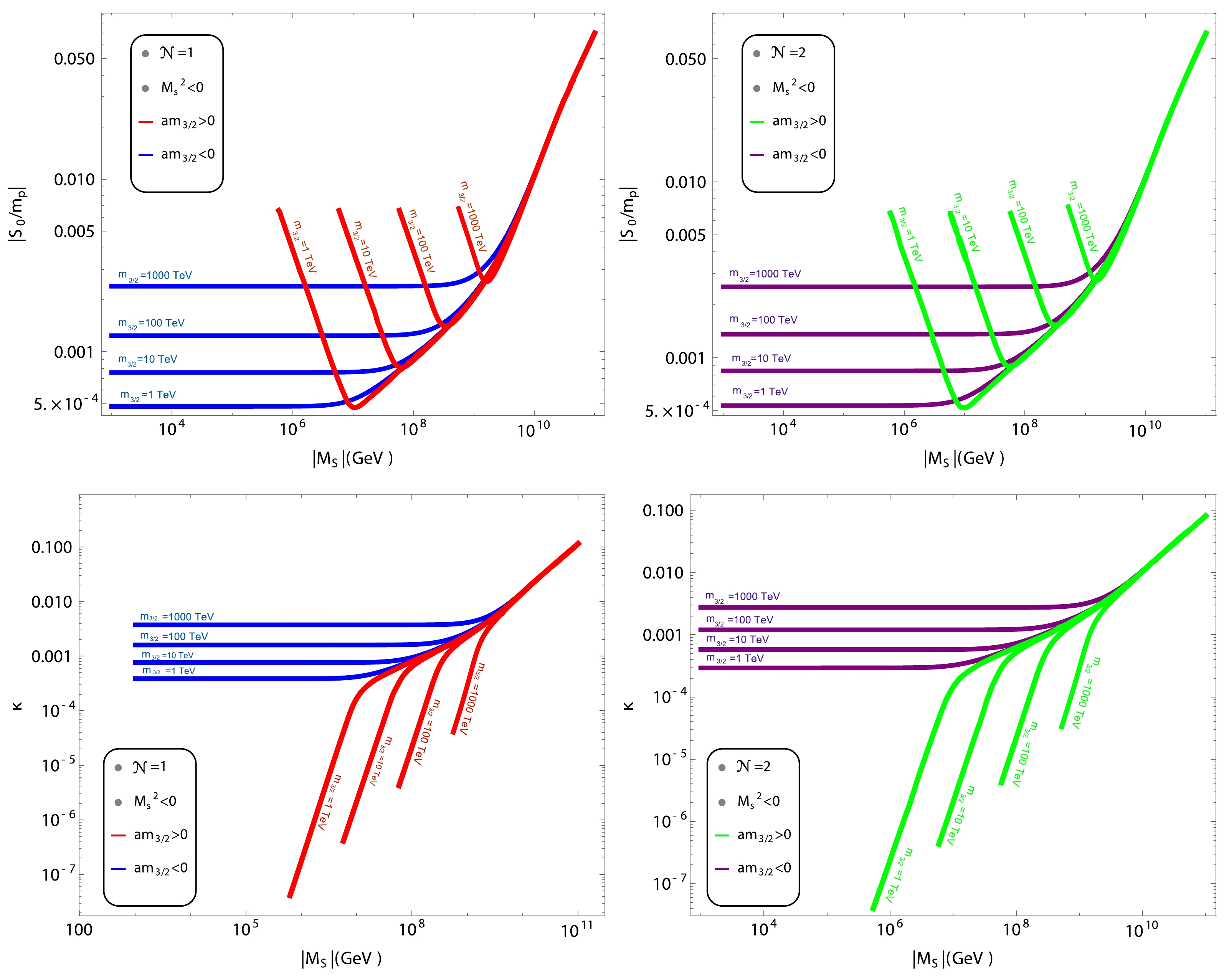

Figure 4.(color online) Plots of $ |M_{S}|-|S_{0}|/m_{p} $ (upper panels) and $ |M_{S}|-\kappa $ (lower panels) planes. Color coding is the same as inFig. 3.

In the upper panel ofFig. 4, we show our calculations on the $ |M_{S}|-|S_{0}|/m_{p} $ plane, and the lower panel presents plots of $ |M_{S}|-\kappa $ . The color coding is the same as inFig. 3. From the upper panel, we see that the maximum variation in $ |S_{0}|/m_{p} $ is from $ 5\times 10^{-4} $ to $ 0.005 $ for a variation in $ |M_{S}| $ between $ 10^{6} $ GeV and $ 10^{7} $ GeV. Other ranges of $ |S_{0}|/m_{p} $ with different values of $ m_{3/2} $ are also shown with the maximum value of $ 0.005 $ . In the lower panel, we also note that the value ofκvaries between $ 10^{-7} $ to $ 10^{-2} $ with variations in $ |M_{S}| $ in the mass interval of $ 10^{6} $ GeV to $ 10^{9} $ GeV for both and green curves. One can also note that, in bothFig. 3andFig. 4, for $ |M_{S}|\gtrsim 10^{10} $ GeV, there is no difference in results between $ am_{3/2}>0 $ and $ am_{3/2}<0 $ .

In addition to the above calculations, we aim to estimate the values of the Hubble parameter during inflationHin these models. In the slow-roll limit, the Hubble parameter depends on the value ofVand is given as

and we calculate it at the pivot scale. InFig. 5, we show the values of the Hubble parameter in the ( $ n_{s}-H $ ) plane. Here, we show our calculations for $ {\cal{N}} $ =1 and $ {\cal{N}} $ =2 as blue and purple lines, respectively. We observe that, with a 2σvariation from the $ n_{s} $ central value,Hvaries almost linearly from $ 9.9\times 10^{7} $ GeV to $ 1.68 \times 10^{8} $ GeV. In the context of the modified swampland conjecture and TCC, it is difficult to satisfy the TCC for SUSY hybrid inflation with minimalKas the TCC requires $ H<1 $ and $ r\sim10^{-31} $ , which are very small values; moreover, the modified swampland conjecture, requires c or $ c^{\prime} $ on the order of 1, which can easily be satisfied for the $ c^{\prime} $ case. To satisfy both conjectures simultaneously, we briefly discuss SUSY hybrid inflation with non-minimalK, where both largerand smallrsolutions are achievable.

Figure 5.(color online) Plot of the $ H-n_s $ plane with $ {\cal{N}}= $ 1 (blue curve), $ {\cal{N}}= $ 2 (purple curve), and $ N_{0}= $ 50.

The non-minimal Kähler potential may be expanded as

Using Eqs. (1), (5), and (24) along with the radiative correction and soft mass terms, we obtain the following inflationary potential:

where

where $ \gamma _{S}=1-\dfrac{7\kappa _{S}}{2}+2\kappa _{S}^{2}-3\kappa _{SS} $ , and we keep the terms up to $ {\cal{O}}\; (\left(\vert S \vert / m_P \right)^4) $ from SUGRA corrections.

and

In the following discussion and numerical calculations, we are mostly interested in the largersolution, modified swampland conjecture, and TCC. Therefore, we consider the solution in which the quadratic term is positive and the quartic term has a negative potential. We further assume soft masses, $am_{3/2}= M_S= 1~ {\rm TeV}$ , withahaving a negative sign.

The signature of the tensor signal primarily manifests in the degree scales of the CMBB-mode polarization. Several past and ongoing experiments are focused on measuring theB-mode power spectrum. The tensor-to-scalar ratio,r, which characterizes the amplitude of primordial gravitational waves, is expected to be measured with high precision by upcoming observational efforts. The Simons Observatory [56] aims for a precision of $ \delta r = 0.003 $ , while CMB-S4 [57] targets a detection of $ r \gtrsim 0.003 $ at more than 5σsignificance or an upper limit of $ r < 0.001 $ with 95% confidence if undetected. LiteBIRD [27] is designed to measurerwith an uncertainty of $ \delta r = 10^{-3} $ . Similarly, PICO (Probe of Inflation and Cosmic Origins) [58] aims to detect $ r = 5 \times 10^{-4} $ at a significance level of 5σ. Additional missions include CORE (Cosmic Origins Explorer) [59], which is projected to exhibit sensitivity toras low as $ 10^{-3} $ ; PIXIE (Primordial Inflation Explorer) [60], which anticipates to measure $ r < 10^{-3} $ at the 5σlevel; and PRISM (Polarized Radiation Imaging and Spectroscopy Mission) [61], which aspires to achieve detection ofras low as $ 5 \times 10^{-4} $ at 5σ.

For our calculations shown inFig. 6, we assume soft masses $ am_{3/2}= M_S= 1 $ TeV, withahaving a negative sign. We display our calculations for $ {\cal N}= $ 1 (blues curves) and $ {\cal N}= $ 2 (purple curves). We set $ n_{s}= $ 0.9665 (central value) and the number ofe-folding $ N_{0}= $ 50. In these figures, all the solutions have sub-Planckian field values. From the left panel ofFig. 6, we note thatκhas large values $ [0.015,0.25] $ for $ \kappa_{S} $ ranges of $ [-0.05,-0.041] $ (blue curve); we also note thatκhas a range of $ [0.01,0.25] $ with $ \kappa_{S} $ in the range of $ [-0.044,-0.038] $ (purple curve). The large values ofκalso implies large values ofr. This can be understood from the relation $ r \simeq \left( \dfrac{2 \kappa^2}{3 \pi^2 A_s (k_0)} \right) \left( \dfrac{M}{m_P} \right)^4 $ given in [52]. This relation implies that, since we have $ M=2\times 10^{16} $ GeV, for large values ofκ, we also have large values ofr. For the previously mentioned ranges of $ \kappa_{S} $ , from the right panel, we see that the maximum value ofris approximately $ 0.01 $ for both $ {\cal{N}}= $ 1 and $ {\cal{N}}= $ 2, and it can be as small as $ 10^{-5} $ . The significant tensor modes predicted by the model are potentially measurable by forthcoming CMB experiments such as LiteBIRD [27], Simons Observatory [56], PRISM [61], CMB-S4 [57], CORE [59], and PIXIE [60].

Figure 6.(color online) Plots forκ(top left panel), tensor to scalar ratior(top right panel), $ \kappa_{SS} $ (middle left panel), and $ \gamma_{S} $ (middle right panel) with respect to non-minimal coupling $ \kappa_S $ for $ N_0 = 50 $ , GUT symmetry breaking scale $ M=2 \times 10^{16} $ GeV, and $ n_s = 0.9665 $ (central value). Blue lines represent $ {\cal{N}}= $ 1, while purple lines represent $ {\cal{N}}= $ 2.

In the lower left and right panels, we plot $ \kappa_{SS} $ and $ \gamma_{S} $ , respectively, as a function of $ \kappa_{S} $ . Here, note that, with $ \kappa_{S}< $ 0, we do not have solutions for $ \gamma_{S}> $ 0 with $ n_{s}= $ 0.9665. In this case, we have solutions only for $ \kappa_{SS}> $ 0 because, for $ \kappa_{SS}< $ 0, fields become trans-Planckian. From the plot of the $ \kappa_{S}-\kappa_{SS} $ plane, we see that, for $ {\cal{N}}= $ 1 and $ {\cal{N}}= $ 2, we have almost the same range of $ \kappa_{SS} $ $ [0.4,2] $ for two different ranges of $ \kappa_{S} $ , that is, from $ -0.049 $ to $ -0.041 $ (blue curve) and from $ -0.044 $ to $ -0.038 $ (purple curve). In contrast, in the $ \kappa_{S}-\gamma_{S} $ plot, we see that, for similar ranges of $ \kappa_{S} $ , $ \gamma_{S} $ varies from –5 to –0.02 for $ {\cal{N}}= $ 1 and $ {\cal{N}}= $ 2. Finally,Fig. 7shows the variation of $ |S_{0}|/m_{p} $ with respect to $ \kappa_{S} $ (left panel) and $ \gamma_{S} $ (right panel). From the right panel, we see that, when $ \kappa_{S} $ varies between $ -0.049 $ and $ -0.041 $ , $ |S_{0}|/m_{p} $ varies between $ 0.06 $ and $ 1 $ . We see from the right panel that $ |S_{0}|/m_{p} $ varies between $ 0.06 $ and $ 1 $ when we change $ \gamma_{S} $ from $ -5 $ to $ 0 $ .

Figure 7.(color online) $ \vert S_0 \vert / m_P $ versus non-minimal coupling $ \kappa_S $ (left panel) and $ \gamma_S $ (right panel). Color coding is the same as inFig. 6.

In addition to the basic inflationary predictions, we discuss the bounds on the parameter space from the swampland conjecture as shown inFig. 8. In the left panel, we show the $ n_{s} $ vs. $ -c^{\prime} $ plane, and in the right panel, we plot the $ \sqrt{2\epsilon} $ vs. $ \sqrt{\alpha/N_{sp}} $ plane. The swampland conjecture imposes a lower bound on the tensor to scaler ratioras expressed in Eq. (22). The details of this bound are provided below ² . Recall that $ -c^{\prime} $ is actually ourη. We calculate $ -c^{\prime} $ at the pivot scale. Therefore, the range of $ -c^{\prime} $ at the pivot scale is $ (-0.023,-0.01 ) $ . Moreover, the inflation ends at $ \eta(x_{e})=-1 $ . Thus, $ -c^{\prime} $ has a range from the pivot scale to the end of inflation, which is $ (-0.023,-1) $ for different values of $ {\cal{N}} $ . FromFig. 8(left panel), it is clear that the value of $ -c^{\prime} $ varies from –0.021 to –0.011, which does not correspond to an $ O(1) $ number. As discussed previously, according to Dvaliet al. [48], the parameterαis related to parameterc, proposed by Vafa et al. [39], as $ \sqrt{\alpha}=c $ . However, in contrast toc, which is a $ O(1) $ parameter, $ \sqrt{\alpha} $ can be any number $ < 1 $ . As discussed in Section 3, $ \sqrt{\alpha}=c=\sqrt{2\epsilon(x_{0})} $ . Notably, according to Eq. (18), any one of the two conditions can be satisfied to maintain consistency with the modified swampland conjecture. Therefore, following Eqs. (18) and (22), we present our calculations in the right panel ofFig. 8. Here, we see that $ \sqrt{{\alpha}/N_{sp}} $ and $ \sqrt{2\epsilon(x_{0})} $ are on the order of $ 10^{-11} $ and $ 10^{-7} $ , respectively; thus, our results are consistent with the modified swampland conjecture for both $ {\cal{N}}= $ 1 and $ {\cal{N}}= $ 2 for minimal SUSY hybrid inflation. InFig. 9, we show our calculations for the swampland conjecture employing the non-minimal SUSY hybrid inflation model with $ N_{0}=50 $ . We see that, with a variation of $ \sqrt{2\epsilon} $ between 0.002 to 0.04, $ \sqrt{\alpha/N_{sp}} $ changes from $ {\cal O}(10^{-6}) $ to $ {\cal O}(10^{-5}) $ , which is consistent with the swampland conjecture.

Figure 8.(color online) Plots for $ n_{s} $ vs. $ -c^{\prime} $ (left panel) and $ \sqrt{\alpha/N_{sp}} $ vs. $ \sqrt{2\epsilon(x_{0})} $ for the minimal case. Color coding is the same as inFig. 6.

Figure 9.(color online) Plots for $ \sqrt{\alpha/N_{sp}} $ vs. $ \sqrt{2\epsilon(x_{0})} $ for $ {\cal{N}} $ =1 (blue curve) and $ {\cal{N}} $ =2 (purple curve) for the non-minimal case.

The TCC imposes an upper bound of approximately $ 10^9 $ GeV on the energy scale during inflation, or equivalently, an upper bound of $ H \leq 1 $ GeV on the Hubble scale during (slow-roll) inflation. To briefly discuss the TCC, we consider the potential up to 26 quartic terms by applying delicate cancellations between the $ \kappa_{S} $ and $ M_{S} $ terms; thus, the remaining potential behaves similar to that in the inflection-point inflation (IPI) scenario. Here, we consider the leading order terms for analytical clarity; otherwise, higher-order terms distort the inflection-point inflation. Fine-tuning the parameters for higher-order terms is necessary to maintain these results, which we derive as shown below. By consider the amplitude of primordial perturbation $ A_{s} $ with the tensor-to-scalar ratior, we can findκin terms ofrand $ A_{s} $ . Similarly, the delicate cancellations between the $ \kappa_{S} $ and $ M_{S} $ terms give us a relation between $ \kappa_{S} $ and $ M_{S} $ , which reads as

Here,rrepresents the value of the tensor-to-scalar ratio at the pivot scale. The scalar spectral index $ n_s $ is defined in Eq. (12) for the smallrsolution; thus, we can write $ n_{s} $ andras follows:

Using above two equation, we can obtain a relation betweenrand $ n_{s} $ at the pivot scale:

The benchmark points for the TCC are listed inTable 1. Points 1, 2, and 3 show the consistency of the solutions with TCC bounds on energy density $E_{\rm inf}$ and scale of inflationH. ³

	Point 1	Point 2	Point 3
$M /{\rm GeV}$	$ 2\times10^{16} $	$ 2\times10^{16} $	$ 2\times10^{16} $
$M_{S}/{\rm GeV}$	0.1	0.1	0.1
$ \kappa_{S} $	0.472509	0.0472509	$ 0.00472509 $
κ	$ 8.86\times 10^{-16} $	$ 8.86\times 10^{-16} $	$ 8.89\times 10^{-15} $
$ \gamma_{s} $	−85.2687	−85.2687	−85.2687
$ N_{0} $	45.363	44.212	44.2117
$am_{3/2}/{\rm GeV}$	0.0000137383	0.0000434442	0.000137383
$E_{\rm inf}/{\rm GeV}$	$ 5.95\times 10^8 $	$ 1.06\times10^9 $	$ 1.88\times 10^9 $
$H/{\rm GeV}$	0.0484924	0.153346	0.484924
$ n_{s} $	0.9655	0.9655	0.9655
r	$ 9.63\times 10^{-32} $	$ 1\times10^{-30} $	$ 1\times10^{-29} $

Table 1.Bench mark points of the TCC. The inflaton field at the pivot scale $ x_{0} $ is close to $ x_{e} $ , which is close to 1.

In this study, we revisited supersymmetric (SUSY) hybrid inflation in light of CMB experiments and swampland conjectures. We first showed that, when radiative and soft mass corrections are applied to the scalar potential, along with SUGRA corrections, supersymmetric hybrid inflation remains consistent with Planck 2018 data despite the impression that it does not. Usually, in SUSY hybrid inflation with minimal Kähler potential, the gauge symmetry breaking scaleMturns out to be $ {\cal O}(10^{15}) $ GeV, which causes the proton decay rate problem. In this study, we presented a new parameter space where the proton decay rate problem could be mitigated by achieving anMof approximately y $ 10^{16} $ GeV with $ M_{S}^{2}< $ 0 and $ am_{3/2}> $ 0. In this scenario, one requires a soft SUSY breaking scale $ |M_{S}| \gtrsim 10^{6} $ GeV. Additionally, we found that the tensor to scalar ratiorwas in the range of $ 10^{-16} $ to $ 10^{-6} $ , which is relatively small. The modified swampland conjecture held, whereas the TCC was difficult to satisfy. Therefore, we also considered non-minimal Kähler potential. We fixed the spectral index $ n_{S}= $ 0.9665 (central value) of Planck 2018 data and $ M=2\times 10^{16} $ GeV and presented our calculations. We showed that, with $ M_{S}= $ 1 TeV, $ m_{3/2}= $ 1 TeV, and $ \kappa_{S}<0 $ for $ {\cal{N}}= $ 1 and $ {\cal{N}}= $ 2,rranges from $ 10^{-5} $ to $ 0.01 $ . We also presented a parametric space and a benchmark point table for SUSY hybrid inflation with non-minimal Kähler potential, showing consistency with the modified swampland conjecture and TCC. The largerrsolutions were only viable outside the strict confines of the TCC, as the TCC imposes stringent constraints on inflationary dynamics. Specifically, within the TCC framework, the tensor-to-scalar ratiormust be extremely small, which is beyond the scope of ongoing and future planned experiments.

We would like to thank Gia Dvali for fruitful discussion. We would also like to thanks to Qaisar Shafi and Mansoor Ur Rehman for their valuable insights at the beginning of the project. Their discussions were particularly beneficial during the calculations.