Generated genuine tripartite steering and its monogamy in the background of a Kerr-Newman black hole

The concept of steering, first proposed by Schrödinger [1] in his response to the Einstein, Podolsky, and Rosen (EPR) paper, is opposed to the complete description of reality provided by quantum mechanics [2]. The objection, known as the EPR paradox, arises from quantum entanglement between two spatially separated particles, indicating that we can use the local measurements on one particle to steer the state of another distant particle. This extraordinary property, known as "spooky action at a distance," suggests a violation of local realism in entangled quantum systems and refers to a measurement process in quantum mechanics in which we cannot relate objective physical reality to entangled quantum systems independent of our chosen measurements. The EPR paradox was demonstrated experimentally for the first time via nondegenerate parameter amplification in a continuous variable system [3]. This method has been successfully applied to the investigation of EPR steering in various continuous variable systems [4−7]. Unlike quantum entanglement, which remains symmetric under the permutation of the parties involved, EPR steering is essentially a directional form of quantum correlation. This means that the steerability from Alice to Bob may not equal that in the reverse direction [8].

Black holes, the densest objects in the universe, are solutions to the Einstein field equations in general relativity. Recently, an increasing number of astronomical observations have both indirectly and directly confirmed their existence [9−15]. Black holes constantly attract physicists from a variety of backgrounds, spanning from astroparticle physics and cosmology to general relativity and quantum field theory in curved spacetime. Because they create the ultimate gravitational environment, black holes are considered prime candidates for studying the mechanisms of quantum gravitational effects in their presence [16,17]. Interestingly, the Hawking radiation caused by black hole evaporation results in the famous black hole information paradox, for which researchers in the entire field are seeking a solution [18−23]. This is a conflict that exists between general relativity and quantum theory and leads to the development of relativistic quantum information. Quantum correlation and coherence have been widely studied in the context of Schwarzschild black holes [24−43]. However, quantum steering has not been studied in Kerr-Newman spacetime. In this study, one of our aims is to investigate the influence of the Hawking effect of the Kerr-Newman black hole on quantum steering. Quantum steering has richer properties than quantum entanglement in curved spacetime. Therefore, another aim is to gain a more complete understanding of the Kerr-Newman black hole through quantum steering.

In this study, we investigate the generated genuine tripartite steering (GTS), redistribution, and monogamy of Gaussian steering in the presence of a four-dimensional Kerr-Newman black hole. Our model includes three modes: modeAobserved by Alice at an asymptotically flat region, modeBobserved by Bob close to the event horizon of the Kerr-Newman black hole, and modeBobserved by anti-Bob in the interior region of the black hole. We find that the gravitational effect of the Kerr-Newman black hole can generate GTS among Alice, Bob, and anti-Bob. The GTS depends on the angular momentum, polar angle, and charge of the black hole. We also find that the "sudden death" ofA→Bsteering leads to the "sudden birth" ofB→Bsteering. This is powerful evidence for the monogamy of quantum steering in Kerr-Newman spacetime, which we demonstrate as follows: partyBcannot be individually steered by partiesAandB, but the collectivityABcan steer partyB. It is worth noting that the condition for maximal steering asymmetry is exactly the transition point between two-way and one-way steering in the Kerr-Newman black hole.

The paper is organized as follows. In Sec. II, we briefly introduce the definition and measure of Gaussian quantum steering and GTS. In Sec. III, we introduce the Hawking effect of the Kerr-Newman black hole, described as a Gaussian channel. In Sec. IV, we study the redistribution of Gaussian steering and its monogamy in the presence of the Kerr-Newman black hole. Finally, Sec. V presents the conclusions.

In this section, we provide a brief introduction to the definition and measurement of quantum steerability for continuous variables. We consider a bipartite continuous variable quantum system described by (n+m) bosonic modes [44]. This bipartite state comprises two subsystems: one observed by Alice withnmodes, and another by Bob withmmodes. For each modei, the corresponding phase-space variables can be denoted by $\hat{a}^{A}_{i}= ({\hat{x}^{A}_{i}+i\hat{p}^{A}_{i}})/{\sqrt{2}}$ and $\hat{a}^{B}_{i}=({\hat{x}^{B}_{i}+ { i}\hat{p}^{B}_{i}})/{\sqrt{2}}$ . These phase-space variables are grouped for convenience into the vector $\hat{R}=(\hat{x}^{A}_{1},\hat{p}^{A}_{1},\cdots,\hat{x}^{A}_{n},\hat{p}^{A}_{n},\hat{x}^{B}_{1},\hat{p}^{B}_{1},\cdots,\hat{x}^{B}_{m},\hat{p}^{B}_{m})^{\rm T}$ , which satisfies the canonical commutation relations $[\hat{R}_{i},\hat{R}_{j}]={\rm i}\Omega_{ij}$ , with $ \Omega=\bigoplus\limits_{1}^{{n+m}} \left(\begin{array}{*{20}{c}} 0\qquad&1\\ -1\qquad&0 \end{array}\right) $ representing the symplectic form. The properties of the Gaussian state are determined entirely by the first and second statistical moments of the quadrature operators. The latter is a covariance matrix with elements $\sigma_{ij}={\rm Tr}[\{\hat{R}_{i},\hat{R}_{j}\}_{+}\rho_{AB}]$ , which can always be arranged in block form,

Here, the submatricesAandBrepresent the covariance matrices corresponding to the reduced states of Alice's and Bob's subsystems, respectively. We emphasize that the covariance matrix $ \sigma_{AB} $ can be described by a physical quantum state if and only if the bona fide uncertainty principle relation

is satisfied.

In terms of Williamson's theorem [45], the symmetric matrix $ M^{B}_{\sigma} $ is diagonalized by a symplectic transformation $ S_{B} $ such that $S_{B}M^{B}_{\sigma}S^{\rm T}_{B}={\rm{diag}}\{\bar{\nu}^{B}_{1},\bar{\nu}^{B}_{1},\cdots,\bar{\nu}^{B}_{m},\bar{\nu}^{B}_{m}\}$ , where $ \{\bar{\nu}^{B}_{j}\} $ are the symplectic eigenvalues of $ M^{B}_{\sigma} $ . Subsequently, the quantification of theA→Bsteerability can be ascertained as [46]

This is the GaussianA→Bsteerability, exhibiting immutability under local symplectic operations. It attains nullity if and only if the state delineated by Eq. (1) remains nonsteerable through Gaussian measurements. In other words,A→Bsteerability quantifies the extent to which the condition in Eq. (3) deviates from fulfillment through Alice's measurement. For a specific covariance matrix $ \sigma_{AB} $ ,A→Bsteerability can take the specific form

where $ S{(\sigma)}=\dfrac{1}{2}\ln(\det \sigma) $ is the Rényi-2 entropy [47]. Furthermore, the GaussianB→Asteerability can be defined by interchanging the components ofAandBin Eq. (4).

For the three-mode Gaussian state $ \sigma_{ABC} $ , the monogamy of quantum steering satisfies the following CKW-type inequalities [48]:

The left hand side of the inequalities shows that the 2 → 1 steering $ {\cal{G}}^{ij\rightarrow k}(\sigma_{ijk}) $ describes how the collectivity $ \{ij\} $ steers the partk, and the 1 → 2 steering $ {\cal{G}}^{i\rightarrow jk}(\sigma_{ijk}) $ describes how the partisteers the collectivity {jk}, wherei,j, andkdenote the different permutations ofA,B, andC. The right hand side quantifies the total bipartite steering. The residual tripartite steering can be defined as the non-negative difference between these two forms of steering, minimized over all possible choices of the probe subsystem [48]. The residual steering for the three-mode system represents the GTS, which is determined by

The minimum in Eq. (6) is always achieved by decomposition.

Einstein's equations yield four well-established, precise solutions for black holes. Among them, Kerr and Kerr-Newman black holes exhibit angular momentum and undergo rotation around one of their axes of symmetry. If a massive spinning star undergoes collapse, it could lead to the formation of a rotating black hole. Given that a significant number of stars exhibit rotation, it is predicted that the majority of black holes also possess rotational characteristics. Now, the Kerr-Newman metric [49−51] in Boyer-Lindquist coordinates can be expressed as

wheret, $ r \in(-\infty,+\infty) $ , $ \varphi \in[0,2\pi) $ , $ \theta \in[0,\pi) $ , $ \Delta=r^{2}+a^{2}- 2Mr + r Q^{2} $ , $ \sum=r^{2}+a^{2}\cos^{2}\theta $ ,Mis the gravitational mass,ais the angular momentum per unit mass, and $ Q^2 = p^2 + q^2 $ , with magnetic chargepand electric chargeq. When both the parametersaandQbecome zero, the Kerr-Newman metric simplifies to the Schwarzschild metric. The widely recognized understanding is that the time-radial part of the geometry of all black holes can be approximated by two-dimensional Rindler spacetime near their horizons [52,53], where the proper acceleration is directly proportional to the surface gravity. These approximations arise inside $ h_{-} $ (cauchy horizon) and outside $ h_{+} $ (event horizon) in the context of the Kerr and Kerr-Newman scenarios. The radii of these horizons correspond to the roots of $ \Delta $ , specifically denoted as

and a corotating coordinate system $ \{t,r,\theta,\widetilde{\varphi}_{\pm}\} $ can be linked to each horizon $ h_{\pm} $ . Corotating azimuthal angles are defined by

with

Because we are studying the time-radial part of the metric, we consider $ \widetilde{\varphi}_{\pm}=\rm{const} $ , so that $ {\rm d}\widetilde{\varphi}=0 $ and

Now, we introduce a new spatial coordinate, denoted asz, in such a way that it becomes zero at the horizon radius $ r=r_{\pm} $

Employing Eqs. (9) and (10), the initial term in the metric can be expressed as [54]

where $ \Sigma_{\pm}=r^{2}_{\pm}+a^{2}\cos^{2}\theta $ . Thus, the time-radial part of the metric takes the form

where

In the vicinity of $ r_{\pm} $ [54], $ f(r,\theta) $ can be formulated as

where the surface gravities $ \kappa_{\pm} $ at $ r_{\pm} $ read as

In terms of the proper time $ t_{\pm} $ of an observer positioned at $ r=r_{\pm} $ , the line element $ {\rm d}l^{2} $ takes the form

where $ f_{0}=f(r_{0},\theta) $ , and ${\rm d}t_{\pm}=\sqrt{f_{0}}{\rm d}t$ . Finally, near the event horizon, that is, $ r\sim r_{+} $ , we choose

and we then obtain

which represents the metric of Rindler spacetime, with its acceleration parameter designated as $ \dfrac{\kappa_{+}}{\sqrt{f_{0}}} $ , where

This suggests that we can model the Kerr-Newman metric near the event horizon using a Rindler metric, with the acceleration parameter representing the proper acceleration of an observer situated at $ r_{0} $ , a point in close proximity to the event horizon.

The particle annihilation and creation operators for Rindler spacetime are described as $ b_{\sigma} $ and $ b^{\dagger}_{\sigma} $ , respectively. Here, the subscript $ \sigma $ = I or II distinguishes between the two causally disconnected Rindler wedges, I and II, arising from the presence of an event horizon in the spacetime. The Minkowski operators $ a^{\dagger}_{R} $ and $ a_{R} $ can be expressed in terms of the Rindler operators $ b^{\dagger}_{\sigma} $ and $ b_{\sigma} $ by Bogoliubov transformations:

where $ \hat{U}=\exp[\eta(b^{\dagger}_{I}b^{\dagger}_{II}-b_{I}b_{II})] $ . Then, the Minkowski vacuum state $ |O_{R}\rangle_{M} $ seen by the Rindler observer, that is, Bob, is given by $ |O_{R}\rangle_{M}=\hat{U}(|O\rangle_{I}\bigotimes|O\rangle_{II}) $ . Here, $ |O\rangle_{I} $ and $ |O\rangle_{II} $ are the Rindler vacuum states of regions I and II, respectively, regarding Bob [32,55].

Near the event horizon $ h_{+} $ , the Kerr-Newman metric reduces to the Rindler metric with the acceleration parameter $ \dfrac{\kappa_{+}}{\sqrt{f_{0}}} $ . The Hartle-Hawking vacuum state of Kerr-Newman spacetime can be expressed in terms of the Boulware Fock space basis using the expression

where $ \tanh \eta=\exp\left(-\dfrac{\pi\sqrt{f_{0}}\omega}{\kappa_{+}}\right) $ , and $ \hat{U}=\exp[\eta(b^{\dagger}_{I}b^{\dagger}_{II}- b_{I}b_{II})] $ is the two-mode squeezing operator. Note that the squeezing transformation $ \hat{U} $ is a Gaussian operation that preserves the Gaussianity of the input states. A symplectic phase-space representation of the two-mode squeezing operation $ \hat{U} $ has the form

where $\cosh \eta=\dfrac{1}{\sqrt{1-{\rm e}^{{-2\pi\sqrt{f_{0}}\omega}/{\kappa_{+}}}}}$ . Based on the analysis provided earlier, the Kerr-Newman metric near the event horizon can be approximated to resemble the Rindler metric. Consequently, an observer in close proximity to the Kerr-Newman black hole's horizon is akin to an observer in close proximity to the Rindler horizon.

We initially consider a two-mode squeezed state shared by Alice and Bob in Minkowski spacetime, which has the covariance matrix

wheresis the squeezing parameter [55]. After sharing, Bob moves toward the event horizon $ h_{+} $ , that is, $ r = r_{0} \sim r_{+} $ . Thus, we consider the following relation:

Therefore, $ \cosh \eta $ can be rephrased as $ \cosh \eta= $ ${1}/{\sqrt{1-{\rm e}^{{-2\pi\omega}/{\kappa}}}}$ , with $\kappa= {\kappa_+}\Big/{\sqrt{\tfrac{(R-1)\left(R-{r_{-}}/{r_{+}}\right)}{R^{2}+{a^{2}\cos^{2}\theta}/{r^{2}_{+}}}}}$ . Here, Bob approaches the event horizon that isR→ 1 ( $ r_0\rightarrow r_{+} $ ); thus, the strength of the gravitational effect of the Kerr-Newman black hole is the greatest. Note that the strength of the gravitational effect increases asRdecreases because Bob is closer to the event horizon, leading to a stronger gravitational effect. However, Alice remains stationary in an asymptotically flat region. The transition from the Minkowski mode to the black hole mode is associated with a symplectic transformation $ S_{B\bar{B}} $ in the phase-space. ModeB, under such a transformation, is mapped into two sets of modes: modeBoutside the event horizon of the black hole and modeBinside the event horizon. Therefore, a complete description of the Gaussian system involves three modes: modeAdescribed by Alice, modeBdescribed by Bob, and modeBdescribed by anti-Bob, a hypothetical observer confined inside the event horizon. The covariance matrix of the Gaussian state describing the complete system is given by [55]

where $ \big[\sigma_{AB}(s)\oplus I_B\big] $ is the initial covariance matrix for the entire Gaussian state. The diagonal elements in Eq. (28) take the forms

where $ I_2 $ denotes the unity matrix in 2 × 2 space. The non-diagonal elements have the following forms:

and

where $ Z_2 $ denotes the third Pauli matrix. The GTS, quantified by the residual steering in Eq. (6), is found to be

Figure 1(a) shows the specific form. For any nonzero values ofsand $ \eta $ , the residual steering is nonzero. This reveals that the state $ \sigma_{AB\bar{B}} $ is genuinely steerable and contains GTS among Alice, Bob, and anti-Bob. We can compute the bipartite steerings in different 2 → 1 and 1 → 2 partitions of the state given in Eq. (28), which are found to be

Figure 1.(color online) (a) Genuine tripartite steering. (b)−(d) 2 → 1 steering and 1 → 2 steering.

The specific form is plotted inFig. 1(b)−(d). As shown in Eq. (32), $ {\cal{G}}^{AB\rightarrow \bar{B}} $ and $ {\cal{G}}^{A\bar{B}\rightarrow B} $ depend on the gravitational parameter $ \eta $ and are different from $ {\cal{G}}^{A\rightarrow B\bar{B}} $ .

Figure 2shows the gravitational influence of the Kerr-Newman black hole on GTS and 2→1 steering. As shown inFig. 2, GTS and 2→1 steering increase with decreasingR. This indicates that the gravitational effect of the Kerr-Newman black hole generates GTS.Fig. 2(a)−(c) demonstrate that the steering increases with the squeezing parameter $ s $ , indicating that the quantum resources shared in the initial state predominantly influence quantum steering. As shown inFig. 2(d)−(f), when Bob approaches the pole of the black hole, that is, the location where the ergosphere touches the event horizon ( $ \theta=0 $ ), GTS and 2→1 steering are greater than in the situation where he reaches the equator ( $\theta= {\pi}/{2}$ ).Fig. 2(g)−(l) interestingly show that, for a black hole with a smaller angular momentum andQ(both magnetic and electric charges), the steering is stronger.

Figure 2.(color online) GTS and 2→1 steering as functions ofRfor different parameters. (a)−(c) We fixM=1,Q=0.997M, $ a=\dfrac{1}{20}M $ , $ \theta=0 $ , and $ \omega=\dfrac{3}{4\pi} $ . (b)−(f) We fixs=1,M=1,Q=0.997M, $ a=\dfrac{1}{20}M $ , and $ \omega=\dfrac{3}{4\pi} $ . (g)−(i) We fixs=1,M=1, $ \theta=0 $ , $ a=\dfrac{1}{20}M $ , and $ \omega=\dfrac{3}{4\pi} $ . (j)−(l) We fixs=1,M=1, $ \theta=0 $ , $ Q=\dfrac{1}{20}M $ , and $ \omega=\dfrac{3}{4\pi} $ .

To better understand the interplay between initial squeezing and the different parameters of the black hole in the degradation and generation of Gaussian steering, we now discuss the behavior of 1 → 1 bipartite steering in the tripartite system. Owing to the causal disconnection between the exterior and interior regions of the black hole, Alice and Bob are unable to access modeBinside the event horizon. Taking the trace over modeB, we obtain the covariance matrix $ \sigma_{AB}(s,\eta) $ as

Employing Eq. (4), we obtain an analytical expression ofA→BGaussian steering as

To check whether the quantum steerability is symmetric in Kerr-Newman spacetime, we define Gaussian steering asymmetry as

where

InFig. 3, we plot the Gaussian steering $ {\cal{G}}^{A\rightarrow B} $ and $ {\cal{G}}^{B\rightarrow A} $ and the steering asymmetry $ {\cal{G}}^{\Delta}_{AB} $ as functions ofR. As shown inFig. 3,A→Bsteering first decreases rapidly and then suffers from a "sudden death" with decreasingR. However, $ B \rightarrow A $ steering only disappears at the limit of $ R\rightarrow 0 $ . $ B \rightarrow A $ steerability is always larger thanA→Bsteerability, indicating that the black hole mode steering the Minkowski mode is easier than the Minkowski mode steering the black hole mode. We find that $ {\cal{G}}^{A\rightarrow B} \neq {\cal{G}}^{B\rightarrow A} $ for anyR, which means that the Hawking radiation of the black hole disrupts steering symmetry. Moreover, the parameter setting that maximizes the steering asymmetry of the state $ \sigma_{AB} $ is $s= {\rm{arccosh}} \left[{\cosh^{2}\eta}/{(1-\sinh^{2}\eta)}\right]/2$ . This condition is similar to that whenA→Bsteering experiences "sudden death." We can choose $\theta= {\pi}/{2}$ and a larger squeezing parameter, angular momentum, electric charge, and magnetic charge to weaken Hawking radiation, thereby enhancing quantum steering.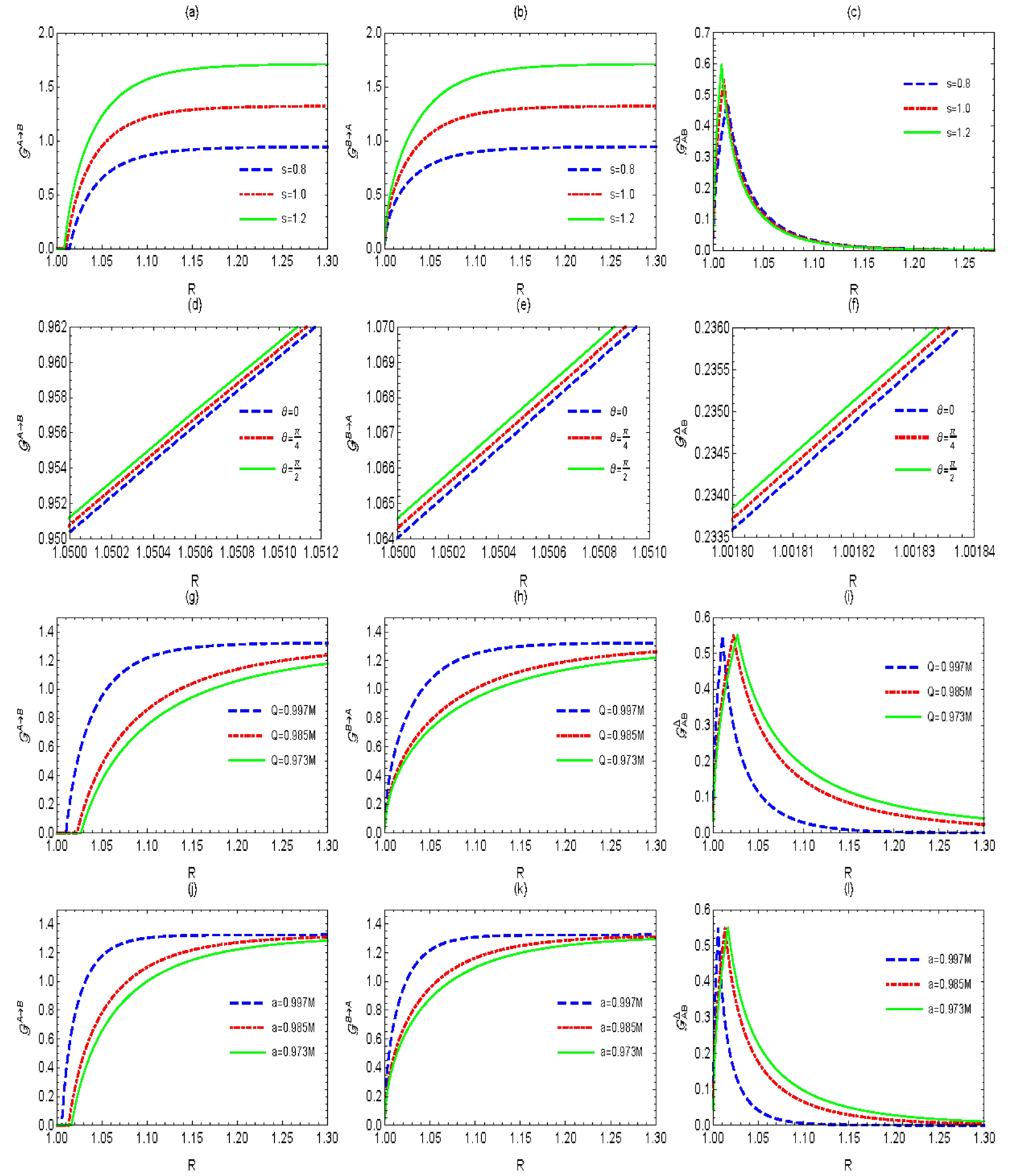

Figure 3.(color online) Steering and its asymmetry between Alice and Bob as functions ofRfor different parameters. (a)−(c) We fixM=1,Q=0.997M, $ a=\dfrac{1}{20}M $ , $ \theta=0 $ , and $ \omega=\dfrac{3}{4\pi} $ . (b)−(f) We fixs=1,M=1,Q=0.997M, $ a=\dfrac{1}{20}M $ , and $ \omega=\dfrac{3}{4\pi} $ . (g)−(i) We fixs=1,M=1, $ \theta=0 $ , $ a=\dfrac{1}{20}M $ , and $ \omega=\dfrac{3}{4\pi} $ . (j)−(l) We fixs=1,M=1, $ \theta=0 $ , $ Q=\dfrac{1}{20}M $ , and $ \omega=\dfrac{3}{4\pi} $ .

We then study the steering between modesAandB, and tracing over the mode inB, we obtain the covariance matrix $ \sigma_{A\bar{B}}(s,\eta) $ for Alice and anti-Bob:

The analytical expressions of steering from modesAtoBand from modesBtoAare found to be

We are also interested in the steering between modesBandB. Tracing over modeA, we obtain the covariance matrix $ \sigma_{B\bar{B}}(s,\eta) $ for Bob and anti-Bob:

Using Eq. (4), we obtain the analytical expressions of $ B\rightarrow \bar{B} $ and $ \bar{B}\rightarrow B $ steering as

The Gaussian steering asymmetry between Bob and anti-Bob, $ {\cal{G}}^{\Delta}_{B\bar{B}}=|{\cal{G}}^{B\rightarrow \bar B}-{\cal{G}}^{\bar B\rightarrow B}| $ , can be computed in a similar manner.

InFig. 4, we plot the Gaussian steering $ {\cal{G}}^{B\rightarrow \bar{B}} $ and $ {\cal{G}}^{\bar{B}\rightarrow B} $ , and the Gaussian steering asymmetry $ {\cal{G}}^{\Delta}_{B\bar{B}} $ as functions ofR. As shown, Hawking radiation can generate quantum steering between Bob and anti-Bob with decreasingR. We observe that the steering from Bob to anti-Bob is nonzero for anyR, whereas the steering from anti-Bob to Bob experiences a "sudden birth" behavior with decreasingR. InFig. 4, we find that $\theta= {\pi}/{2}$ and a larger squeezing parameter, angular momentum, electric charge, and magnetic charge are not conducive to Hawking radiation generating steering. The condition of maximal steering asymmetry is interestingly found as $s= {\rm{arccosh}} \left[{\cosh^{2}\eta}/{(1-\sinh^{2}\eta)}\right]/2$ , indicating that $ \bar{B}\rightarrow B $ steering experiences "sudden birth."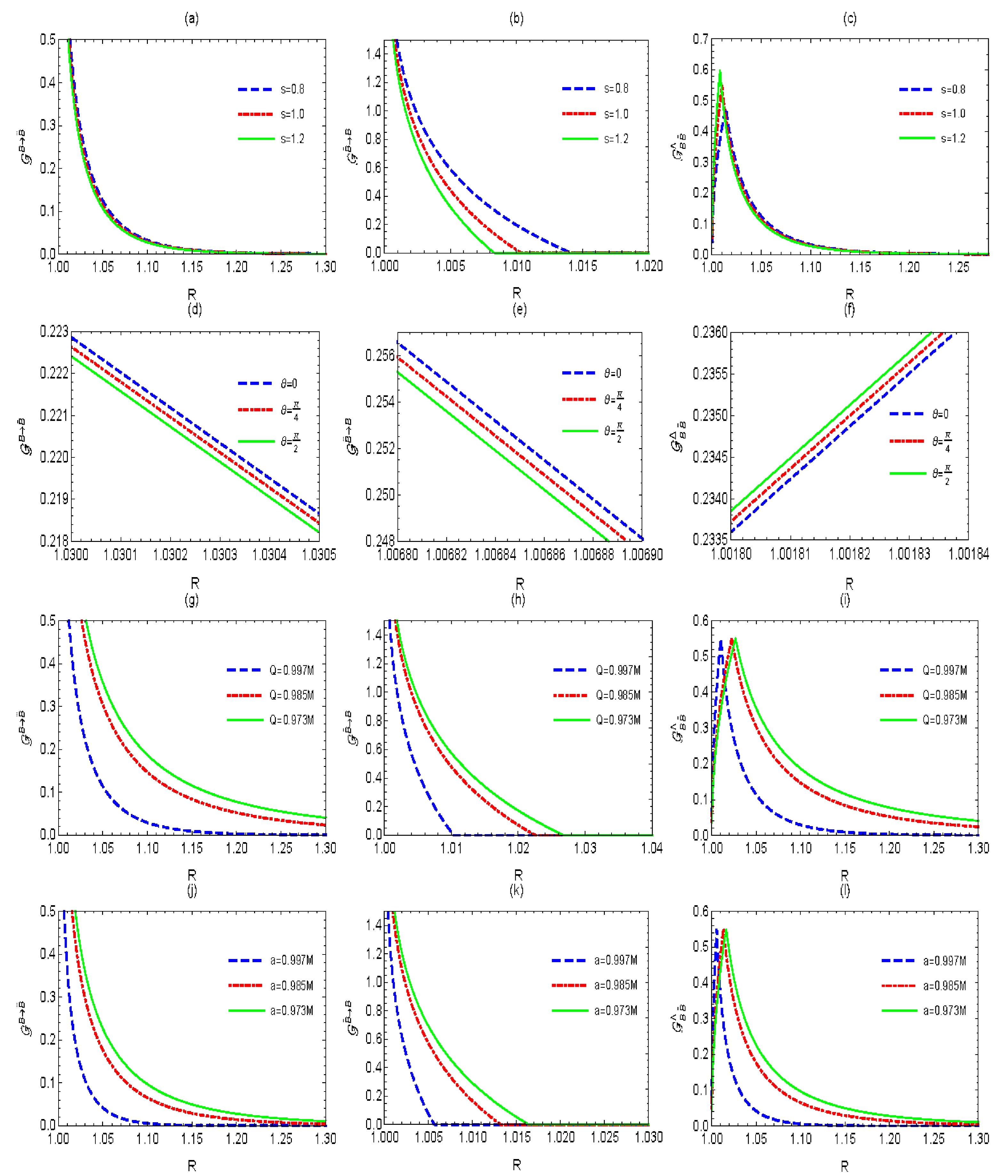

Figure 4.(color online) Steering and its asymmetry between Bob and anti-Bob as functions ofRfor different parameters. (a)−(c) We fixM=1,Q=0.997M, $ a=\dfrac{1}{20}M $ , $ \theta=0 $ , and $ \omega=\dfrac{3}{4\pi} $ . (b)−(f) We fixs=1,M=1,Q=0.997M, $ a=\dfrac{1}{20}M $ , and $ \omega=\dfrac{3}{4\pi} $ . (g)−(i) We fixs=1,M=1, $ \theta=0 $ , $ a=\dfrac{1}{20}M $ , and $ \omega=\dfrac{3}{4\pi} $ . (j)−(l) We fixs=1,M=1, $ \theta=0 $ , $ Q=\dfrac{1}{20}M $ , and $ \omega=\dfrac{3}{4\pi} $ .

Can quantum steering be freely distributed within the tripartite system in Kerr-Newman spacetime? Similar to entanglement monogamy, steering monogamy has very attractive explanations: $ x \rightarrow yz $ steering is always greater than the sum of $ x\rightarrow y $ and $ x\rightarrow z $ steering for all three sets of directions in Kerr-Newman spacetime. As shown inFig. 5, with decreasingR,A→Bsteering experiences "sudden death," whereas $ \bar{B} \rightarrow B $ steering experiences "sudden birth." Furthermore, the "sudden death" point is in accordance with the "sudden birth" point. Note that, steering monogamy exists in a more extreme scenario: (i) partiesAandBcannot individually steer partyB, but the collectivity {AB} can be steered by the measurements performed on Bob's side; (ii) partiesBandBcannot steer partyAindividually, but the collectivity {AB} can steer partyA; and (iii) partiesAandBcannot steer partyBindividually, but the collectivity {AB} can steer partyB. In particular, owing to the limitation of steering monogamy, the "sudden death" ofA→Bsteering leads to the "sudden birth" ofB→Bsteering under the influence of Hawking radiation. In other words, the limitation of steering monogamy means thatAandBcannot steerBsimultaneously in Kerr-Newman spacetime. Specifically, if $ {\cal{G}}^{A\rightarrow B}>0 $ holds true, $ {\cal{G}}^{\bar B\rightarrow B}=0 $ (and vice versa) for the tripartite system $ \sigma_{AB\bar B} $ . This is powerful evidence for steering monogamy in Kerr-Newman spacetime.

Figure 5.(color online) (a) Steering monogamy for the condition of $ \eta < \eta_{0} $ $ (\eta_{0}={\rm{arccosh}} \sqrt{1+\tanh^{2}(s)} $ . (b) Steering monogamy for the condition of $ \eta > \eta_{0} $ .

The generated GTS, redistribution, and monogamy of Gaussian steering are investigated in the presence of a four-dimensional Kerr-Newman black hole. We consider three subsystems: subsystemAobserved by Alice at an asymptotically flat region, subsystemBobserved by Bob close to the Kerr-Newman black hole's outer horizon, and subsystemBobserved by anti-Bob inside the event horizon. We find that the gravitational effect of the Kerr-Newman black hole can generate GTS among the three subsystems. This dependence is observed on factors such as the polar angle, angular momentum, electric charge, and magnetic charge of the black hole. Furthermore, 2 → 1 and 1 → 2 steering are symmetric, whereas 1 → 1 steering is asymmetric in four-dimensional Kerr-Newman spacetime.

The "sudden death" of the steering from Alice to Bob leads to the "sudden birth" of the steering from anti-Bob to Bob under the influence of the gravitational effect. This is powerful evidence for the monogamy of quantum steering in Kerr-Newman spacetime, suggesting that this monogamy can regulate the redistribution of quantum steering in curved spacetime. We observe that a critical point $ \eta_{0}={\rm{arccosh}} \sqrt{1+\tanh^{2}(s)} $ occurs at the condition of maximal steering asymmetry, marking the transition between two-way and one-way steering, or between the phenomena of "sudden death" and "sudden birth" in Kerr-Newman spacetime.