Holographic Einstein ring of a charged Rastall AdS black hole with bulk electromagnetic field

Investigating the expanding nature of our universe can be defined as the study of evolution, comprising a vast array of experimental and productive changes that have occurred across all of time and space, from the big bang to the emergence of humankind. In recent years, General Relativity (GR) [1] has prevailed as the most successful description of gravitational interaction. Indeed, Einstein's GR possesses astonishing predictions that have been observed throughout the years, such as the discovery of super-massive black holes (BHs) at the center of galaxies [2−5] and the detection of gravitational waves [6,7], which have fundamentally altered the way we perceive and test the accelerated expansion of our universe. Nevertheless, GR has been shown to have some shortcomings based on observational data, such as the discovery of the late-time accelerated expansion of the universe found through Type Ia supernovae [8,9], or from a theoretical perspective [10]. For the last twenty years, scientists have focused on theoretical and observational efforts so that the understanding of humanity regarding this phenomenon of the universe may be improved. From a theoretical perspective, it is well-known that this theory entails some open questions, such as the cosmological constant problem [11] or the coincidence problem [12], which led us to seek a more general theory of gravity. Moreover, GR encapsulates singularities,e.g., the primordial Big Bang singularity, which are still puzzling to the research community, and a quantum description of gravity is required for a comprehensive analysis [10].

To tackle the abovementioned problems, one can consider the modified theories of gravity (MTG) that provide a foundation for the current understanding of the physical phenomena occurring in the universe [13]. An extensive study regarding MTG conducted by many researchers showed that these theories are not only capable of dealing with dark energy (DE) problems but also with the inflationary epoch [14]. Some of the MTG include $ f(R) $ , $ f(R,T) $ , $ f({\cal{T}}) $ , and $ f({\cal{Q}}) $ gravity (whereRis the Ricci scalar,Tis the trace of energy-momentum tensor, $ {\cal{T}} $ is the torsion scalar, and $ {\cal{Q}} $ is the non-metricity scalar) [15−19], and many others have been suggested in the last few decades. In GR, the coupling between space-time geometry and matter is minimal, leading to the conservation law of energy-momentum tensor, which is valid only for flat space-time. In this scenario, an interesting modification of GR was proposed by Rastall in $ 1972 $ [20], and nowadays, it has become a prominent theory of gravity because it is presented as an MTG with non-conserved energy-momentum tensor and measures the affinity of the space-time geometry to couple with matter field in a non-minimal manner. In this proposal, Rastall confronted the usual conservation law of energy-momentum tensor (i.e., $ \nabla_{\alpha}T^{\alpha\beta} = 0 $ , $ \nabla_{\alpha} $ is the covariant derivative)) in curved space-time.

In fact, this conservation law ( $ \nabla_{\alpha}T^{\alpha\beta} = 0 $ ) may be violated in curved space-time. By considering this restriction of the conservation law, Rastall introduced a special amendment in GR by improving the usual conservation law as $ \nabla_{\alpha}T^{\alpha\beta} = \lambda R^{,\beta} $ , whereλis a coupling parameter of Rastall gravity (RG) [20]. For the case $ \lambda = 0 $ , Einstien's GR can be recovered. Another important feature of RG is that the field equations are relatively simpler than the other MTG and hence easier to handle. However, the field equations of RG are quite simple, and they appear to be consistent with some observational data on the Hubble parameter and age of the universe [21], meaning that it could be free of the entropy and the problems of the standard cosmology [22]. Also, RG provides good agreement with experimental observations of the matter-dominated phase against Einstein's GR [23]. Observational data associated with helium nucleosynthesis also satisfy RG [24]. More studies on the cosmological features of RG, including its consistency with numerous cosmic phases, are introduced in [25]. In addition, RG has been discussed in the framework of the Gödel-type universe with a perfect fluid matter, and it was found that the geodesics of particles do not alter [26].

Besides, some attention has been focused on debating whether RG is equivalent to GR. In this context, Visser claimed that RG is a rearrangement of the matter sector of Einstein's GR [27]. In the context of non-equilibrium thermodynamics (for homogeneous and isotropic flat Friedmann-Lemaître-Robertson-Walker background model), Daset al. [28] concluded that generalized RG is equivalent to Einstein's GR. On the contrary, Darabi et al. [29] disagree with Visser's claim, and they concluded that Visser misinterpreted the matter-geometry coupling term, which led him to the wrong conclusion. From this perspective, they further showed that by applying Visser's method to $ f(R) $ theory, one may derive that RG is equivalent to GR, which is not true. In addition, they indicated that RG is an “open” theory in comparison to GR and is more compatible with observational cosmology. Hansrajet al. [30] also investigated this dispute, and their results are in good agreement with the results obtained by Darabiet al. [29]. They concluded that RG could satisfy the basic conditions for a physically viable model, where GR does not meet the requirements; for details, see Ref. [30]. Hence, RG is not equivalent to GR, which has been proven through many studies [31−33], and it is worth studying because it faces a challenge from cosmological as well as astrophysical observations.

In this scenario, Moradpour and Salako [34] studied the limitation of RG due to the application of the Newtonian limit to the theory. Properties of the traversable asymptotically flat wormhole solutions were studied in [35] within the fabric of RG. Moradpouret al. [36] observed the remarkable differences between RG and GR in cosmological solutions. Moradpouret al. [37] further generalized RG and discussed the accelerated expansion of the universe. In [38], the authors investigated the evolution of gravitational potential in the context of Rastall scalar field theories and concluded that the obtained results indicate consistent scenarios that may emergefrom a Rastall unification model for DE. The observational illustration of RG parameters in static space-times with galaxy-scale strong gravitational lensing was analyzed in [39]. The extension of the standard ΛCDM model in the context of RG was investigated through observational constraints in [40]. The relationship between RG and $ f(R,L_{m}) $ (where $ L_{m} $ is the matter Lagrangian) theory was analyzed in [41], where the authors constrained the Rastall parameter to lie in the range $ \lambda\leq0 $ and $ \lambda\geq1 $ through energy conditions. Moreover, the relation between RG and the k-essence model was analyzed in [42], where the authors claimed that both theories produce similar results. The most successful of these attempts was with the $ f(R,T) $ theory, in which the Lagrangian $ f(R,T) = R+\beta T $ is considered as a Rastall Lagrangian [43]. Inspired by the interesting features of RG, many researchers have analyzed the different cosmological aspects of Refs. [44−51]; several such studies are found in literature.

To reveal the geometrical optics of BH, the newly born field of multi-messenger astronomy employs plasma radiations, gravitational waves, and neutrinos [52]. Historically, the deflection of light due to strong gravitational force around compact objects has been a powerful tool in the verification of GR predictions [53]. Since the light rays travel across the null geodesics of the background metric, the solution of the geodesic equation provides realistic information to unveil the geometry of any body compact enough to hold a critical curve. This is an unstable circular orbit for mass-less particles and corresponds to the backtrack of the light trajectory from the observer's screen that asymptotically approaches a bound photon orbit [54]. In astrophysics, a BH or compact object will typically be surrounded by its accretion disk, which provides the fundamental source of illumination [55]. The term BH shadow has come to interpret the interior of the critical curve. The size and shape of the critical curve are determined by the background geometry, whereas the optical appearance of a compact object is heavily influenced by the astrophysics of the accretion disk. If the disk is optically thin, one expects the optical appearance to be dominated by a central brightness depression, the so-called shadow, surrounded by strongly lensed light rays that have turned many times around the BH close to the critical curve and appear superimposed through direct emission close to the boundary of the shadow [56].

The details of the BH shadow image were confirmed by the Event Horizon Telescope (EHT) [2−5] in $ 2019 $ , where the tracking of the plasma radiations around the super-massive BH in the center of the Messier (M) $ 87 $ elliptical galaxy, modulated by the strong magnetic fields, released a bright ring-shaped lump of radiations surrounding a circular dark region. This picture convincingly confirms the existence of BHs in our universe. Furthermore, the results obtained from EHT exhibit the existence of a magnetic field around M $ 87 $ , prompting us to better understand and explain the launching of energetic jets from its core. This carries information about the geometry of the electromagnetic fields responsible for the synchrotron emission and shows that magnetically arrested accretion disks surround M $ 87 $ [57,58]. An astrophysical BH provides a constant space-time structure, illuminated by a time-varying emission region by some external sources of the luminous accretion material, leading the BH to have a variety of shapes and emit a variety of colors. Due to different interesting scenarios of matter accretions around the BHs, the study of BH shadows and their physical characteristics has reached a peak position among the scientific community. Hence, the study of BH shadow configurations not only enables us to comprehend the geometric structure of space-time but also helps us to explore various gravity models in detail.

The anti-de Sitter (AdS)/conformal field theory (CFT) consists of a solid apparatus where strongly coupled field theories are investigated. Any given field theory, including finite temperature, has a hydrodynamical description in the infrared (IR) limit, corresponding to long-length scales. The AdS/CFT correspondence as a concrete realization of the holographic principle explicitly identifies that the theory of quantum gravity in AdS bulk space is equivalent to a dual CFT on the boundary [59]. The dual pair is the most prominent example between type IIB string theory on Ad $ S_{5}\times $ S⁵and the maximally super-symmetric gauge theory in four dimensions, i.e., the $ N = 4 $ super Yang-Mills [60,61] theory. Thus, the holographic principle of gravity obtained the peak position among various fields of physics because it is not only used to indirectly test the correspondence related to quantum physics but also provides solutions to some problems faced by strong coupling systems. From this perspective, the AdS/CFT correspondence is successfully applied in various areas along with the analysis of the strong coupling dynamics of quantum chromodynamics (QCD) and electroweak theories as well as BHs and quantum gravity; the AdS/CFT correspondence is also used to investigate relativistic hydrodynamics or different applications in condensed matter physics, superfluidity, and superconductivity, thus improving our understanding of high-temperature superconducting physics [62−70]. To date, the theoretical aspects of the holographic principle have been of special interest to scientists, and numerous publicationshave been devoted to this subject in the context of MTG [71−77]. Recently, in the context of AdS/CFT correspondence, Kakuet al. [78] proposed a method to create a star orbiting in an asymptotically AdS space-time, and then, they demonstrated the angular position of the star with the help of a lensed response function. Therefore, the AdS/CFT correspondence strongly supports a better understanding of various physical topics.

Because of the above discussion, apart from the study of the shape and size of shadows, the possible observational characteristics of the BH shadow surrounded by different accretion flows were studied for a long time. In the context of RG, Guoet al. [79] investigated the shadows and photons sphere of the charged BH surrounded by a perfect fluid radiation field with the static/infalling accretion flow models and found that the shadow luminosity of this BH with static spherical accretion is brighter than that with infalling spherical accretion. In [80], the authors studied the shadow cast of non-commutative BH in RG and observed that the luminosity of the resulting shadow closely depends on the non-commutative parameter. The shadow of a rotating BH surrounded by an anisotropic fluid field in RG was investigated by Kumaret al. [81]. They found that the rotating Rastall BH leads to a shadow smaller than that of the Kerr BH for a given value of the rotating parameter. Saleem and Aslam [82] investigated the shadow and observable signatures of the non-commutative charged Kiselev BH within different accretion flow models. They observed that the specific intensity of this BH profile was darker in the case of infalling gas compared to a static one due to the Doppler effect. Heet al. [83] discussed the BH shadow within the framework of the clouds of strings and quintessence and found that the brightness distribution of the photon sphere is a normal function of the string attenuation factor. Since then, BH shadows and their relevant phenomenological consequences have been investigated in several publications within the framework of MTG as well as in RG (for example, see Refs. [84−89]).

Although the mentioned literature provides a realistic description of the shadow dynamics simulations of a BH, there is still a need to further understand the geometrical properties, and their associated deeper phenomenological consequences need to be addressed through effective implementations. In the framework of the AdS/CFT correspondence, the holographic image of an AdS BH in the bulk was constructed when the scalar wave emitted by the source at the AdS boundary enters and then propagates in the bulk [90,91]. In particular, the researchers observed the Einstein ring in the holographic framework, and the size of the ring is consistent with the size of the BH photon sphere, which is observed through geometrical optics. Motivated by this, the authors in [92−99] constructed holographic images of AdS BHs in the context of different space-time backgrounds. In all these studies, they investigated the distinct features of Einstein's ring structure in holographic quantum matter and concluded that holographic images can be used as an effective tool to distinguish different types of BHs for fixed wave sources and optical systems. Following the idea given in [90,91], in the present study, we further investigate the Einstein ring structure for the lensed response of the complex scalar field as a probe wave on the charged Rastall AdS BH solution within the framework of AdS/CFT correspondence. We analyze the possible effect of model parameters on the resulting Einstein ring, which further confirms that the appearance of such an Einstein ring structure may be used as a strong signal for the existence of its gravity dual. To achieve this, the remainder of the paper is organized as follows.

In Sec. II, we briefly define the background of charged Rastall AdS BH and the holographic setup with a finite chemical potential. Section III is dedicated to constructing the special optical system and studying the Einstein ring images under the various values of the involvedmodel parameters. A comparison between the resultsobtained by the geometric optics approximation and wave optics is presented in Sec. IV. Finally, Sec. V provides a discussion and concluding remarks.

According to Rastall's proposal, the energy-momentum conservation law is revised as [20]

and the field equations of RG are formulated as

where $ G_{\alpha\beta} $ , $ T_{\alpha\beta} $ , andkare the Einstein tensor, energy-momentum tensor, and Rastall gravitational coupling constant, respectively. In the last few years, RG has begun a new era in gravitational physics, and many works on various BH solutions and related thermodynamics have been investigated in [100−103]. In the framework of RG, we consider the static spherically symmetric BH metric with the electromagnetic field in the cosmological constant background given as [100]

where

where $ f(r) $ is the metric function, which is determined in terms of massMand chargeQ, and ${\rm d}\Omega^{2} = {\rm d}\theta^{2}+\sin^{2}\theta {\rm d}\varphi^{2}$ . The cosmological constant Λ is related to the AdS radiusl, which is defined as $ \Lambda = -\dfrac{3}{l^{2}} $ . For simplicity, hereafter, we set $ l = 1 $ . Further, to analyze the holographic images of the charged AdS BH solution in RG within the framework of AdS/CFT correspondence, we first define the holographic setup of the dual BH images from the response function of the boundary quantum field theory with external sources. Closely following [90,91], for the source $ {\cal{J}}_{{\cal{O}}} $ , we employ a time-periodic localized Gaussian source with frequencyω, on one side of the AdS boundary and scalar waves generated by the source can propagate in the bulk. When the scalar wave propagates inside the BH space-time and reaches the other side of AdS the boundary, the corresponding response function is generated, such as $ \langle O\rangle $ , which gives information about the bulk structure of the BH space-time. A schematic diagram of this setup is shown inFig. 1.

Figure 1.(color online) Schematic diagram of imaging a dual BH.

By using a special optical system, we can convert the extracted response function $ \langle O\rangle $ into the holographic image, which can be seen on a virtual screen. The ( $ 2+1 $ )-dimensional boundary CFT on a $ 2 $ -sphere $ S^{2} $ is naturally dual to a BH in the AdS₄space-time or the massless scalar field in space-time. To achieve the goal, we use a new definition $ v = 1/r $ , which gives $ f(r) = v^{-2}f(v) $ . From this perspective, we revised the metric (3) as follows:

The value of $ v = 0 $ corresponds to the AdS boundary, where the dual quantum system lies. The Hawking temperatureTof the BH is related to its surface gravity, which is calculated as [100]

where $ v_{h} $ is the inverse of the horizon radius of the BH.

The behaviors of temperatureTversus the inverse of the horizon $ v_{h} $ , parameterλ,and chargeQare shown in the left, middle, and right panels ofFig. 2, respectively. FromFig. 2(left panel), we see that when $Q = 0.5, \lambda = 0.01$ , the temperatureThas the maximum value at point ( $v_{h} = 0.0822522,\; T = 3.02991$ ) and then gradually decreases with increasing inverse of the horizon $ v_{h} $ . The middle panel ofFig. 2shows that when $ Q = v_{h} = 0.5 $ , the temperatureThas the lowest value at point ( $\lambda = 0.01, T = 0.534661$ ) and then sharply increases as the strength of the Rastall parameterλincreases. The right panel ofFig. 2shows that when $ v_{h} = 0.5,\; \lambda = 0.01 $ , the temperatureThas the maximum value at point ( $Q = 0.8, T = 0.530782$ ) and then sharply decreases with increasing chargeQ. This feature may be used as a method to distinguish the charged Rastall AdS BH solution from that of previous studies [92−99] and may affect the following response function, which is derived through the holographic setup. Now, we consider the complex scalar field as a probe field in the charged Rastall AdS background. In this regard, the corresponding dynamics are described by the following Klein-Gordon equation [104]: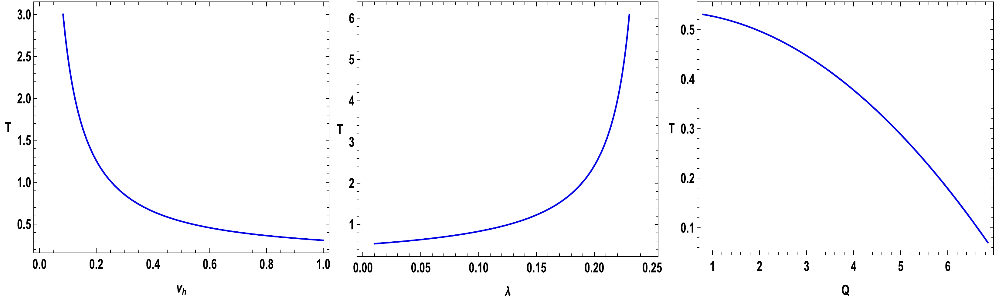

Figure 2.(color online) Relation between temperatureTversus the inverse of the horizon $v_{h}$ (with $Q=0.5,~\lambda=0.01$ ), parameterλ(with $Q=v_{h}=0.5$ ), and chargeQ(with $v_{h}=0.5,~\lambda=0.01$ ), shown in the left, middle and right panels, respectively.

where $D_{\nu}\equiv\nabla_{\nu}-{\rm i}eA_{\nu}$ is the covariant derivative operator,Ais associated with electromagnetic four-potential, Φ interprets the complex scalar field witheas its electric charge, and $ {\cal{M}} $ represents the mass of the scalar field. Further, to solve this numerically in a more convenient manner, we prefer to define the ingoing Eddington coordinate as [92]

and then, the non-vanishing bulk background fields are transformed into the following form:

where $ A(v) = Q(v-v_{h}) $ . In this case, the gauge transformation is also applied to the electromagnetic four-potential. By holography, $ \mu = Qv_{h} $ is denoted as the chemical potential of the boundary system. Here, we take $ {\cal{M}}^{2} = -2 $ for definiteness. With $ \Phi = v\phi $ , the asymptotic behavior of the scalar field close to the AdS boundary can be expressed as

Based on the holographic dictionary, $ {\cal{J}}_{O}(u,\theta,\varphi) $ denotes the external source for the boundary field theory, and the corresponding expectation value of the dual operator, the so-called response function, is defined as [105]

where $ \langle O\rangle $ corresponds to the expectation value of the dual operator when the source is turned off. As defined in [90,91], we choose an axisymmetric and monochromatic oscillating Gaussian wave packet source and fix it at the south pole of the boundary $ {S}^{2} $ ,i.e., $ \theta_{0} = \pi $ as the source. Thus, we have

whereηis the width of Gaussian wave source and $ Y_{n0} $ is the spherical harmonics function. We ignore the Gaussian tail safely due to its smallest value; hence, we only consider the case $ \eta<<\pi $ . Further, the coefficients of the spherical harmonics $ Y_{n0} $ can be written as [91]

Based on Eq. (13), the corresponding bulk solution takes the following form:

where $ V_{n} $ satisfies the equation of motion as

and the asymptotic behavior of $ V_{n} $ can be expressed in the following form:

Similarly, the resulting response $ {\langle O\rangle}_{{\cal{J}}_{O}} $ can be defined as

Then, we have

where $ \hat{\omega} = \omega+e\mu $ . Now, our main purpose is to solve the radial Eq. (16) with a boundary condition such as $ V_{n}(0) = 1 $ at the AdS boundary and the horizon boundary condition on the BH event horizon. From this perspective, we obtain the efficient numerical solution of Eq. (16) through the pseudo-spectral method [92], derive the corresponding numerical solution for $ V_{n} $ , and extract $ {\langle O\rangle}_{n} $ . Then, the total response function $ {\langle O\rangle} $ can be found with the help of extracted $ {\langle O\rangle}_{n} $ and through Eq. (18). Here, we choose some proper values of the considered BH space-time and lens parameters as examples to clearly show that the optical appearance arises from the diffraction of the scalar field of the BH, which can be seen inFigs. 3−5. The amplitude of the total response function is plotted for different values ofλwith $Q = v_{h} = 0.5, \;\omega = 80, e = 1$ , and for different values ofωwith $\lambda = 0.01,\; Q = v_{h} = 0.5, e = 1$ , as shown in the left and right panels ofFig. 3, respectively. Clearly, the left panel ofFig. 3shows that the amplitude is maximum whenλhas smaller values and then decreases with larger values ofλ. Meanwhile, the right panel ofFig. 3shows that the period of the scalar wave is maximum when $ \omega = 30 $ , and it gradually decreases with increasing values ofω. The left panel ofFig. 4illustrates the amplitude of the total response function for different values of electric chargeewith $\lambda = 0.01, Q = v_{h} = 0.5,\; \omega = 80$ . Similarly, the right panel ofFig. 4depicts the amplitude of the total response function for different values ofμwith $\lambda = 0.01,\; v_{h} = 0.5,\; \omega = 80, e = 1$ , where $Q = 0.1,\; 0.5$ , and $ 0.9 $ corresponds to $\mu = $ 1/5, 1, and $ 9/5 $ , respectively. This figure shows that the absolute amplitude of the total response function increases when botheandμhave larger values.Figure 5also depicts the behavior of the amplitude by varying the temperatureTof the boundary system for $\lambda = 0.01,\; Q = 0.5, \omega = 80,\; e = 1$ , where $v_{h} = 0.4, \; 0.5$ , and $ 0.6 $ corresponds to $T = 0.652,\; 0.535$ , and $ 0.458 $ , respectively. From this figure, one can see that the amplitude of the total response function significantly changes with temperatureT; for instance, when $ T = 0.458 $ , the amplitude reaches a peak position and moves down at $ T = 0.535 $ and $ 0.652 $ nicely (seeFig. 5). This implies that the amplitude of the total response function increases with decreasing values ofT. All these results imply that the amplitude of the total response function closely depends on the Gaussian source and space-time geometry. In the next section, we transform this response function as the observed images on the screen, which may be useful to reflect the distinct features of the space-time geometry.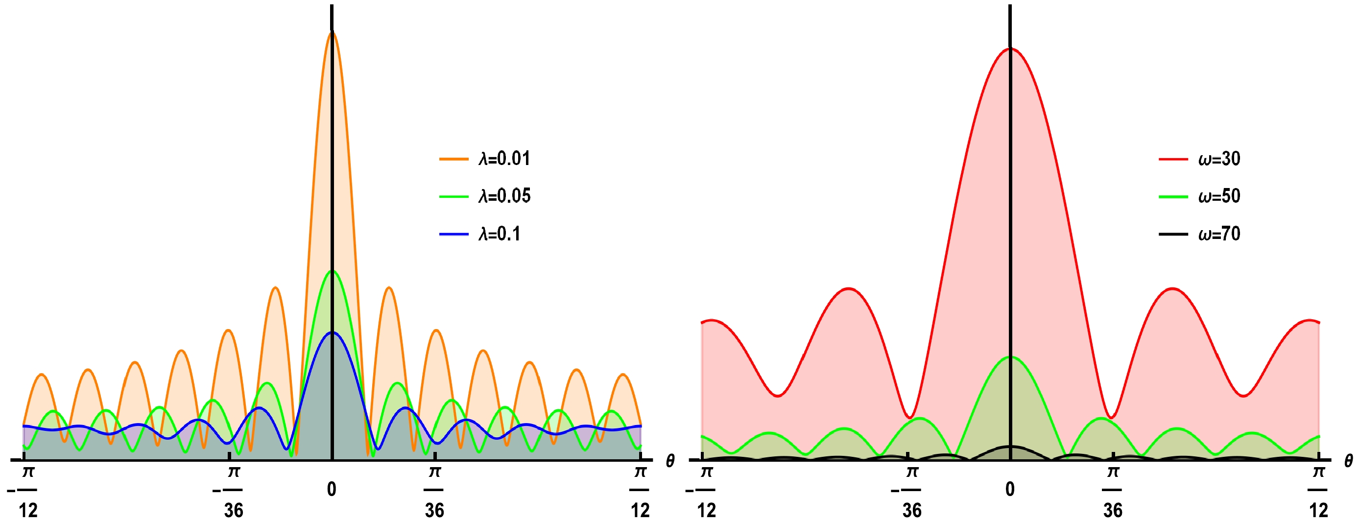

Figure 3.(color online) Absolute amplitude of total response function for different values ofλwith $Q=v_{h}=0.5,\; \omega=80,\; e=1$ (left panel) and for different values ofωwith $\lambda=0.01,\; Q=v_{h}=0.5,\; e=1$ (right panel).

Figure 5.(color online) Absolute amplitude of total response function for different values ofTwith $\lambda=0.01,\; Q=0.5, \; \omega=80, $ $ e=1$ . From top to bottom, the values ofTcorrespond to $v_{h}=0.4,\; 0.5,\; 0.6$ , respectively.

Figure 4.(color online) Absolute amplitude of the total response function for different values ofefor $\lambda=0.01,\; Q=v_{h}=0.5,\; \omega=80$ (left panel) and for different values ofμfor $\lambda=0.01,\; v_{h}=0.5,\; \omega=80,\; e=1$ (right panel). Further, in the right panel, from top to bottom, the values ofμcorrespond to $Q=0.1,\; 0.5,\; 0.9$ , respectively.

After analysis of the physical interpretation of the extracted response function $ {\langle O\rangle} $ , we use it to directly interpret the image of the BH on the screen. As stated in [90,91], to observe the extracted response function $ {\langle O\rangle} $ , we need to introduce a special optical system, which is composed of an extremely thin convex lens and the spherical system shown inFig. 6. In the middle position, there is a convex lens, and we assume the lens is infinitely thin and the size of the lens is much smaller than the focal lengthf, which is regarded as a transform of the plane wave into the spherical waves. Imagine that, from the left side ofFig. 6, the incident wave is irradiated at the lens, and the wave converts to the transmitted wave at the focus, which is depicted on the screen; see the right side ofFig. 6. With the help of this apparatus, we analyze the visual appearance of the holographic Einstein ring image under suitable values of the model parameters, which may help us to deeply understand the actual astrophysical situation of space-time structure and its associated deeper phenomenological consequences.

Figure 6.(color online) Structure of image formation system on the screen.

Let us define an observational point at ( $ \theta, \varphi) = (\theta_{\text{obs}},\; 0 $ ) on the AdS boundary, where an observer is surrounded by a small white circle, as shown in the left side ofFig. 6. We introduce new polar coordinates as ( $ \theta', \varphi' $ ) such that

( $ \theta' = 0,\; \varphi' = 0 $ ), which corresponds to the center of the observation region. For simplicity, we define Cartesian coordinates ( $ x,y,z $ ) with $ (x,y) = (\theta'\cos\varphi',\; \theta'\sin\varphi') $ in the observation region. To develop an optical setup, in the middle position, we fix the convex lens on the ( $ x,y $ )-plane. The focal length and radius of the convex lens are presented byfandd, respectively. Moreover, we adjust a spherical screen having coordinates as $ \vec{x}_{\mathrm{S}} = (x,y,z) = (x_{\mathrm{S}},y_{\mathrm{S}},z_{\mathrm{S}}) $ , satisfying $ x^{2}_{\mathrm{S}}+y^{2}_{\mathrm{S}}+z^{2}_{\mathrm{S}} = f^{2} $ [90,91]. With the help of a convex lens, the incident wave $ \Psi_{\mathrm{in}}(\vec{x}) $ with frequencyωcan be the transmitted in the following form:

where $ \vec{x} = (x,y,0) $ is the coordinate position on the AdS boundary, where the convex lens is placed in the observation range. Then, this wave is considered as the spherical wave and will transform into the observed wave $ \Psi_{\mathrm{sc}}(\vec{x}_{\mathrm{s}}) $ when it is reached on the screen as

whereϖis the distance from the lens point $ (x,y,0) $ to the spherical screen ( $ x^{2}_{\mathrm{S}},\; y^{2}_{\mathrm{S}},\; z^{2}_{\mathrm{S}} $ ), which is defined as [91]

where $ \vec{x}_\mathrm{s} = (x_\mathrm{s}, y_\mathrm{s}) $ . Now, considering the Fresnel approximation $ f\gg |\vec{x}| $ , we obtain

where $ \Xi(\vec{x}) $ is the window function

Based on Eq. (24), we now plot the holographic Einstein ring image on the screen via Fourier transformation. In this way, one can illustrate how the wave source and space-time geometry affect the Einstein ring.

To understand this, we illustrate the density maps of the holographic Einstein ring images on the screen for different values of parameterλand observational angles of the AdS boundary with $ Q = v_{h} = 0.5,\; \omega = 80,\; e = 1 $ (seeFig. 7). From this figure, one can see that when $ \lambda = 0.01 $ and the distant observer is located at $\theta_{\rm obs} = 0^\circ$ , there is a bright ring with a series of concentric striped patterns in the image, which is shown inFig. 7(a). FromFig. 7(a) to7(d), we observe that as the value of the observational angle is increased, the bright ring transforms into a luminosity-deformed ring, instead of a strict axisymmetric ring. In particular, when $\theta_{\rm obs} = 60^\circ$ (seeFig. 7(c)), bright light arcs appear, rather than a bright ring, and further transform into bright light points when $\theta_{\rm obs} = 90^\circ$ , as shown inFig. 7(d). When we increase the parameterλ, such as $ \lambda = 0.06 $ , the same phenomena exist as for $\theta_{\rm obs} = 0^\circ$ . When $\theta_{\rm obs} = 30^\circ$ , we observe that two large light arcs appear, where the right arc is brighter compared to the left one (seeFig. 7(f)). Further, when $\theta_{\rm obs} = 60^\circ$ , the large arcs are changed into small arcs and further converted into two light spots when $\theta_{\rm obs} = 90^{\circ}$ , as shown inFig. 7(g) and7(h), respectively. These findings are also consistent with [90,91]. Next, when we fix $ \lambda = 0.11 $ and vary the positions of the distant observer (seeFig. 7(i) to7(l)), we notice that the optical appearance of the ring behaves almost the same as we discussed in the previous case when $ \lambda = 0.06 $ . However, a significant difference is found in the radius of the ring gradually moving toward the center of the screen, which is more prominent in this case. When the strength of parameterλfurther increases,i.e., $ \lambda = 0.16 $ , we see the series of axisymmetric concentric rings at $\theta_{\rm obs} = 0^{\circ}$ , and these rings are closer to the center of the screen, as shown inFig. 7(m). When $\theta_{\rm obs} = 30^{\circ}$ , we see bright light arcs, and these arcs are changed into pairs of bright light points when $\theta_{\rm obs}$ changes from $\theta_{\rm obs} = 60^{\circ}$ to $\theta_{\rm obs} = 90^{\circ}$ . Further, from top to bottom, we note that as the value of the RG parameterλincreases, the overall brightness of the ring slightly increases, which is difficult to observe.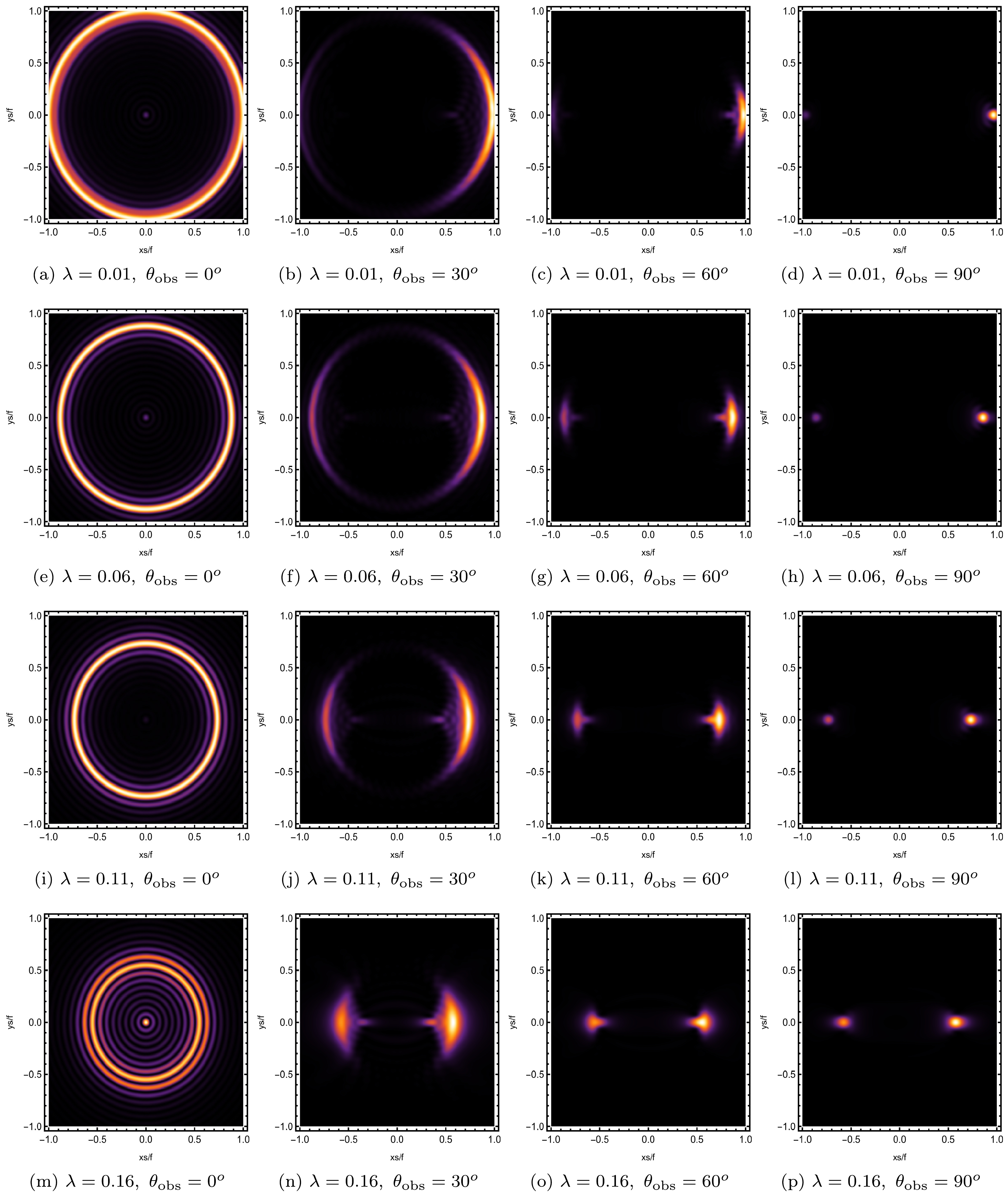

Figure 7.(color online) Density maps of the lensed response on the screen at various observation angles under suitable values ofλwith $Q=v_{h}=0.5,\;\omega=80,\;e=1$ .

Moreover, as shown inFig. 8, we further analyze the influence of the parameterλon the brightness curves with fixed values of $ Q = v_{h} = 0.5,\; \omega = 80 $ , and $ e = 1 $ . Thexand $ -x $ intercepts correspond to the radius of rings, and the vertical axis shows the brightness of the lensed response on the screen. FromFig. 8(a), when $ \lambda = 0.01 $ , it is observed that the peak curves lie close to the boundary, which means that the ring radius has maximum value, and the curves lie at the points $ -1 $ and $ 1 $ on thex-axis. When parameterλgrows,i.e., $ \lambda = 0.06 $ , the peak curves gradually move toward the center and lie at the points $ -0.8 $ and $ 0.8 $ on thex-axis, meaning the ring’s radius decreases. However, the brightness of the lensed response slightly increases in this case (see the vertical axis ofFig. 8(b)). Similarly, inFigs. 8(c) and8(d), we see that the peak curves gradually move toward the center with increasing values of parameterλ. Moreover, a significant difference is found inFig. 8(d) as compared to previous cases, when $ \lambda = 0.16 $ ; in the middle of the screen, there is a peak curve, which shows the maximum value compared to boundary curves. This effect can also be seen inFig. 7(m), where the bright light spot in the center of the screen corresponds to the peak curve ofFig. 8(d). All these results imply that increasing values ofλdecrease the ring’s radius and slightly affect the brightness of the shadow.

Figure 8.(color online) Changes in brightness of the lensed response on the screen for different values ofλat $Q=v_{h}=0.5,~\omega=80,~e=1$ .

Now, we discuss the influence of wave source on the holographic Einstein ring image, which is observed at the position of the north pole,i.e., $\theta_{\text{obs}} = 0^{\circ}$ , as depicted inFig. 9. We selected the values of parameters $\lambda = e = 0.01,\; Q = v_{h} = 0.5$ and plotted four different density maps according to some specific values ofωas an example. To analyze the effect of the wave source, we fix $ \eta = 0.05 $ and $ d = 0.6 $ for the convex lens and note that as the value of the frequency increases, the corresponding ring becomes sharper. Further, for a better understanding of the description of the wave source, we depict the corresponding profiles of the lensed response function inFig. 10under the same set of parameters as mentioned inFig. 9. From this figure, we observe that decreasing values of frequencyωlead to enhancing the gap between the brightness curves as well as increasing the brightness. Based on these profiles, we concluded that the geometric optics approximation provides better configurations about the dual image of the BH in the high frequency limit.

Figure 9.(color online) Density maps of the lensed response on the screen for different values ofωat the observation angle $\theta_{\text{obs}}=0^{o}$ with $\lambda=e=0.01,~Q=v_{h}=0.5$ .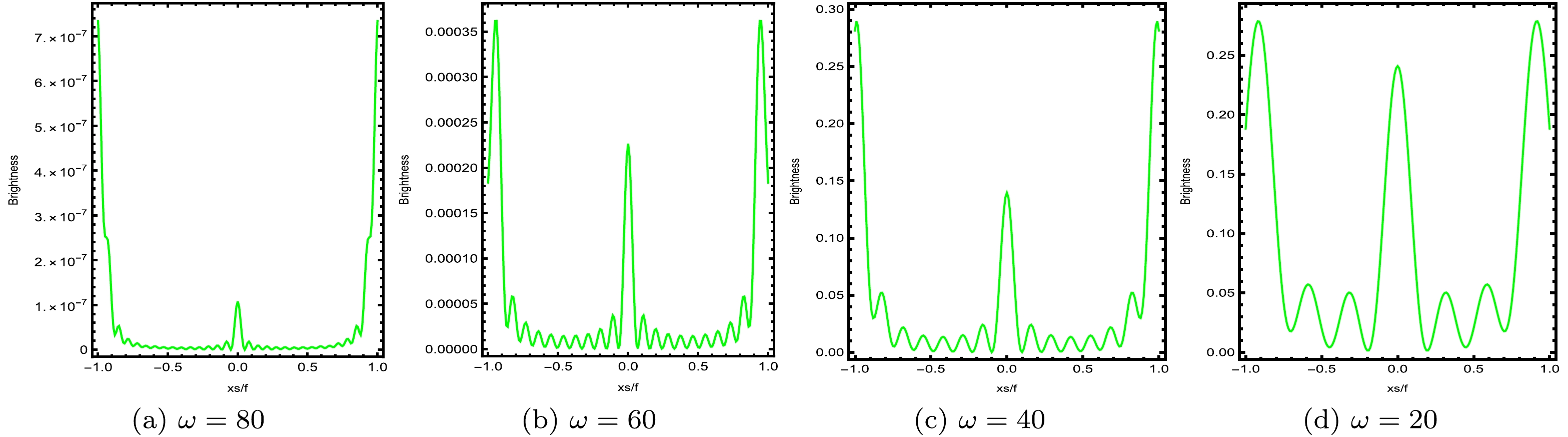

Figure 10.(color online) Changes in brightness of the lensed response on the screen for different values ofωwith $\lambda=e=0.01, $ $ Q=v_{h}=0.5$ .

Now, we are interested in defining the possible effect of the horizon temperatureTon the profiles of the lensed response function, as depicted inFig. 11at the observational angle $\theta_{\text{obs}} = 0^{\circ}$ with a fixed value of chemical potential $ \mu = 1 $ and $ \lambda = e = 0.01,\; \omega = 80 $ . We obtained the values of temperature $ T = 0.0249,\; 0.0746,\; 0.1243,\; 0.174 $ corresponding to charges $ Q = 0.1,\; 0.3,\; 0.5,\; 0.7 $ , respectively. In particular, when $ T = 0.0249 $ , the corresponding ring lies close to the center. As the temperatureTgrows to $ T = 0.0746 $ , the resulting ring moves away from the center. Similarly, when the temperature further grows to $ T = 0.174 $ , the corresponding bright ring is further shifted toward the boundary of the screen (seeFig. 11(d)). This effect can also be seen by going left-to-right on the sequence of images inFig. 12, where the peak curves of the brightness are gradually shifted toward the boundary with increasing temperatureT. Furthermore, when $T = 0.0249, 0.0746,\; 0.1243$ , we see fewer brightness curves in the center of the large curves (seeFig. 12), and corresponding to these curves, we see the bright light spot in the screen, as shown inFig. 11. However, when $ T = 0.174 $ , we see a very dim light spot in the center of the screen, which is difficult to detect (seeFig. 11(d)).

Figure 11.(color online) Density maps of the lensed response on the screen for different values ofTat the observation angle $\theta_{\text{obs}}=0^{\circ}$ with a fixed value of chemical potential $\mu=1$ and $\lambda=e=0.01, ~\omega=80$ . From left to right, the values of temperatureTcorrespond to $Q=0.1,~0.3,~0.5,~0.7$ , respectively.

Figure 12.(color online) Changes in brightness of the lensed response on the screen for differentTwith a fixed value of chemical potential $\mu=1$ and $\lambda=e=0.01, ~\omega=80$ . From left to right, the values of temperatureTcorrespond to $Q=0.1,~0.3,~0.5,~0.7$ , respectively.

Consequently, we further observe the influence of chemical potentialμon the Einstein ring image of AdS BH at the observational angle $\theta_{\text{obs}} = 0^{\circ}$ with a fixed value of temperature $ T = 0.45 $ and $ \lambda = e = 0.01, \; \omega = 80 $ , as shown inFig. 13. FromFig. 13, we note that, when $ \mu = 0.05 $ and $ 0.35 $ , the radius of the Einstein ring does not change and lies almost at the same positions on the screen from the center, indicating that here, the effect of the chemical potentialμon the Einstein ring is negligible. However, as we increase the value ofμto $ \mu = 0.65 $ , as shown inFig. 13(c), the position of the Einstein ring slightly varies and moves toward the center. However, when we fix $ \mu = 0.95 $ , we see that the position of the Einstein ring is dramatically changed and comes closer to the center of the screen sharply (seeFig. 13(d)). These results are also depicted inFig. 14, where we show the changes of the lensed response function on the screen under the same set of parameters mentioned inFig. 13. We observe that the peaks of the curves are slightly changed from $ \mu = 0.05 $ to $ \mu = 0.95 $ , but the positions of the peak curves significantly move toward the center, particularly when $ \mu = 0.95 $ . In summary, we say that smaller values of chemical potentialμhave a negligible contribution to changing the position of the bright ring, whereas large values ofμsignificantly affect it. From this perspective, we conclude that, under this framework, the increasing values ofμlead to decreasing the radius of the bright ring.

Figure 13.(color online) Density maps of the lensed response on the screen for different values of chemical potentialμat the observational angle $\theta_{\text{obs}}=0^{\circ}$ with a fixed value of temperature $T=0.45$ and $\lambda=e=0.01, ~\omega=80$ . From left to right, the values of chemical potentialμcorrespond to $Q=0.0099,~0.0599,~0.0706,~0.0165$ , respectively.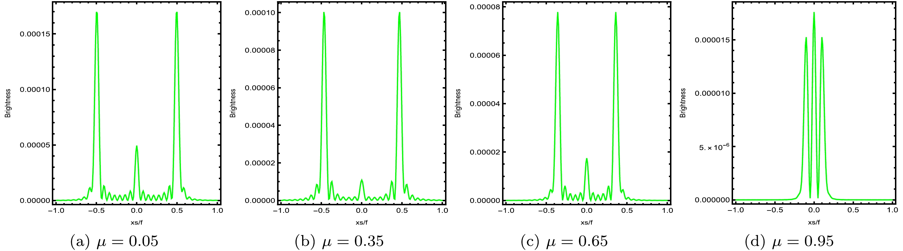

Figure 14.(color online) Changes in brightness of the lensed response on the screen for different values of chemical potentialμwith a fixed value of temperature $T=0.45$ and $\lambda=e=0.01, ~\omega=80$ . From left to right, the values of chemical potentialμcorrespond to $Q=0.0099,~0.0599,~0.0706,~0.0165$ , respectively.

In wave optics, we observe that at the position of the photon orbit, there is the brightest ring in the image. Now, we will analyze this brightest ring in the image through the optical geometry. Thus, to understand the motion of photons around the BH, we need to define the geodesic equations by considering the Hamilton-Jacobi formulation [106]. The dynamics of BH shadows are widely studied by the Lagrangian and Hamiltonian formalisms in the context of different MTG. The usual procedures give two conserved quantities such as energyEand angular momentumLalong the axis of symmetry. Despite presenting the motivation for the Hamilton-Jacobi formulation, we require the Lagrangian for deriving the relation between the constants of motion. From this perspective, the motions of photons in the vicinity of a charged AdS BH are described by a Lagrangian formalism as

where $ \dot{x}^{\mu} $ is the four-velocity of the photon, and ''.'' is the derivative with respect to the affine parameterσalong the geodesics. As we only consider the photons that move on the equatorial plane, we apply the initial conditions as $ \theta = \pi/2 $ and $ \dot{\theta} = 0 $ . Further, the Lagrangian is independent explicitly on timetand azimuthal angleϕ; hence, one can obtain the expressions of two conserved quantities as

As Eq. (27) will be used in further calculations to analyze the motion of photons in a particular space-time through the corresponding geodesics equations, this equation will help in converting the system in terms of the conserved quantities. Now, in the background of the charged AdS BH, the Klein-Gordon equation is reduced to the following Hamilton-Jacobi equation [92,107]:

where $ {\cal{S}} $ is the action. The Hamilton-Jacobi equation is separable, and it possesses a solution of the form

wheretdenotes the time-like coordinate,φparameterizes the orbits of the space-like Killing field, and $ \widehat{R}(r) $ is defined as

The trajectory of geodesics can be further obtained by considering the partial derivatives of $ {\cal{S}} $ with respect tot,φ,andras

The ingoing angle $\theta_{\rm in}$ of the light ray with the normal vector of boundary $ u^{b} = \frac{\partial}{\partial r^{b}} $ is defined as [91]

where $ v^{a} $ is the spatial component of $ 4 $ -velocity of the geodesic, $ g_{ab} $ is the induced metric on $ t = $ constant, and $ |v| $ and $ |u| $ are the norms of $ v^{a} $ and $ u^{b} $ with respect to $ g_{ab} $ , respectively. Moreover, Eq. (32) has the equivalent relation

where $ \widehat{E} $ is considered as the energy of a single particle. Hence, the incident angle $\theta_{\rm in}$ of the photon orbit, which comes from the infinite boundary, satisfies the following relation:

as depicted inFig. 15. This relation is still applicable when the photon is located in the photon sphere. In this scenario, we denote the angular momentum as $ L_{\rho} $ , which is calculated as

Figure 15.(color online) Schematic picture showing the particular ingoing and outgoing angles of the photon revolving around the BH once.

In geometrical optics, when a distant observer near the AdS boundary looks up into AdS bulk, angle $\theta_{\rm in}$ provides information about the angular distance of the image of the ray from the zenith. As there is axisymmetry when both endpoints of the geodesic and the center of the BH are coinciding, the observer will see a circular-shaped image with a radius equal to the incident angle $\theta_{\rm in}$ [90,91]. Further, as presented inFig. 16, one can calculate the angle of the Einstein ring, which is displayed on the screen with radius $ r_{R} $ as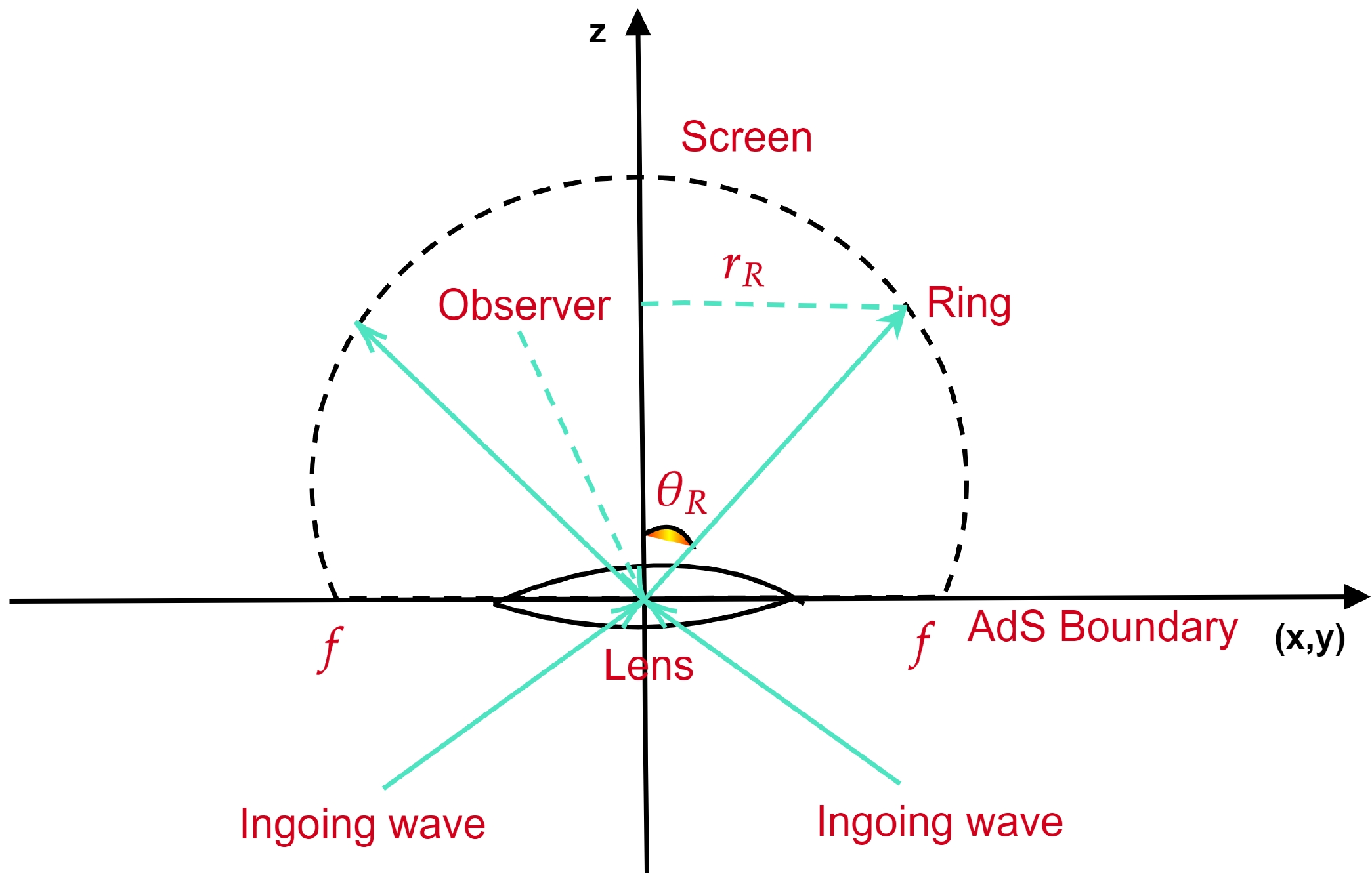

Figure 16.(color online) Schematic picture showing the relation between $\theta_{R}$ and $r_{R}$ .

In addition, when the angular momentum is sufficiently large, such as $\sin\theta_{\rm in} = \sin\theta_{R}$ , we have the following relation [91]:

The incident angle of the photon and angle of the photon ring illustrate the position at which any distant observer can see the clear picture of the photon ring. Next, we will numerically analyze the visual appearance of the corresponding results, which should be essentially equal. InFig. 17, we show the radii of the BH horizon, location of the photon orbit, Einstein radius of the photon orbit, and Einstein ring radius in the unit offas a function of BH horizon $ r_{h} $ for different values ofλ.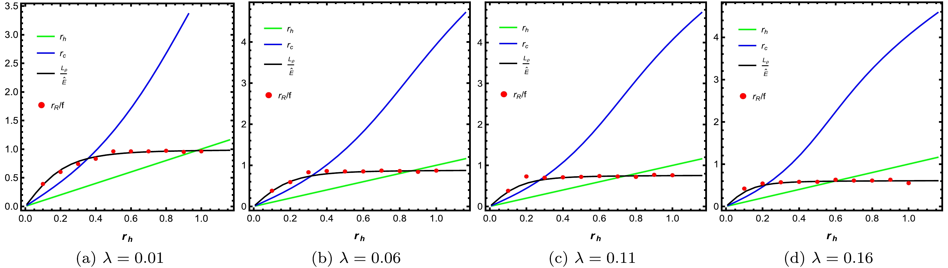

Figure 17.(color online) Plots showing the BH horizon $r_{h}$ , location of photon orbit $r_{c}$ , Einstein radius of the photon orbit (black line), and Einstein ring radius obtained by wave optics (discrete red points) in the unit offfor different values ofλwith fixed values of $\mu=1,~e=0.01$ , and $\omega=80$ .

InFig. 17(a), when $ \lambda = 0.01 $ , we see that the location of the photon ring continuously changes with increasing horizon $ r_{h} $ (see blue curve). Further, we see that the Einstein ring radius appreciably increases at lowervalues of the horizon $ r_{h} $ and then starts to flatten out with respect to the BH horizon $ r_{h} $ (see black curve ofFig. 17(a)). Last, we see that the Einstein ring radius obtained by our holographic method fits well with geometric optics, as discrete red points always lie on the black curve or in its vicinity. Similarly, inFigs. 17(b)−(d), the dependence of the radii of BH horizons $ r_{h} $ , the location of the photon orbit, and the Einstein ring radius obtained by both wave optics and geometric optics on the parameterλare presented. In these graphs, we notice that, with increasing values of parameterλ, the radii of BH horizon $ r_{h} $ and location of the photon orbit $ r_{c} $ increase, and a behavior similar to that discussed forFig. 17(a) is observed. However, a significant difference is also observed; as the values of parameterλincrease from left to right, the Einstein ring radius (black curve) slightly increases at smaller values of the BH horizon $ r_{h} $ and then starts to flatten out throughout the horizon $ r_{h} $ . This effect can be seen more clearly when $ \lambda = 0.16 $ , where the Einstein ring radius starts to flatten out at much smaller values of the horizon $ r_{h} $ compared to previous cases. Lastly, in all cases, the discrete red points, for the Einstein ring radius obtained by our holographic method, always lie on or near the black curve.

For a comprehensive analysis, inFig. 18, we further plot the trajectories of BH horizon radii $ r_{h} $ , location of the photon orbit $ r_{c} $ , Einstein radius of the photon orbit (black curve), and Einstein ring radius in the unit off(discrete red points) as a function of chemical potentialμfor different values ofλ. FromFig. 18(a), whenμhas smaller values, the radii of the BH horizon show the maximum value and then drop sharply with increasing values ofμ. Similarly, the location of the photon orbit and Einstein ring radius gradually change with respect to increasing values ofμ. Moreover, the Einstein ring radius, which is obtained through the holographic method (see discrete red points), lies on or around the black curve, indicating that our results obtained by wave optics fit well with those by geometric optics. InFig. 18(b) and18(c), we observe that the radii of BH horizon and location of the photon orbit behave similarly, as defined in the previous case. However, it is observed that when $ \lambda = 0.06 $ , at smaller values ofμ, the discrete red points are slightly shifted away from the black curve and exactly lie on the curve when $ \mu\sim0.7 $ and then slightly shifted away from the black curve. Similarly, when $ \lambda = 0.11 $ , this effect can be seen more clearly; for example, at initial values ofμ, the discrete red points are significantly shifted away from the black curve, but when $ \mu\sim0.5 $ , these points closely lie on the black curve or its surroundings. Hence, in this case, whenλhas smaller values, such as, $ \lambda\in[0.01,0.06] $ , the discrete red points lie close to the black curve. Finally, the credibility of the brightest holographic ring in the image obtained using wave optics is supported by its consistency with that predicted by geometric optics.

Figure 18.(color online) Plots show the BH horizon $r_{h}$ , location of photon orbit $r_{c}$ , Einstein radius of the photon orbit (black line), and Einstein ring radius obtained by wave optics (discrete red points) in the unit offfor different values ofμwith fixed values of $T=0.37,~e=0.01$ , and $~\omega=80$ .

The study of BH space-times is a prominent topic among the GR and MTG research communities. Significant information on gravitational, thermodynamics, and quantum effects in curved space-time can be revealed through BHs. In the past few years, considerable progress in theoretical and observational explorations of BHs has been observed. These findings opened a new era in gravitational physics triggered by the leap in quantity, quality, and variety of observational data from different probes. Recent collaborations, such as the EHT, have shown that it is feasible to carry out observations of super-massive BHs with near horizon scale resolution. This allows us to directly study the gravitational lensing effect in the strong gravity regime, where we expect the peculiarities of different space-times to become apparent in the images. To this end, strong gravitational lensing is an important observational tool for probing the space-time geometries around massive objects, where the optical appearance of the photon sphere provides a concrete description of space-time configurations. Motivated by this, in this study, we investigated the Einstein ring structure for the lensed response of a complex scalar field as a probe wave propagating in the charged Rastall AdS BH in the framework of AdS/CFT correspondence. In general, real quantum materials are engineered at a finite chemical potential. Thus, for a better understanding of this, we need to consider the bulk electromagnetic field; hence, the BH should be charged.Figure 2(left panel) shows that the temperature gradually decays with respect to the inverse of the horizon $ v_{h} $ . Meanwhile, it gradually increases with increasing RG parameterλ(see middle panel ofFig. 2). Moreover, the right panel ofFig. 2shows that the temperatureThas the maximum value when charge $ Q = 0.8 $ and then sharply decreases with increasing chargeQ. These results imply that the Hawking temperature closely depends on the parameterλas well as the BH horizon $ v_{h} $ . This distinct feature of the horizon temperature may be used as a tool to differentiate the charged Rastall BH solutions from those of other studies [92−99].

The nature of the absolute amplitude of the total response function for different values of the involved parameters is illustrated inFigs. 3to5, which show the corresponding behavior of the wave oscillations according to the variation in state parameters. The left plot ofFig. 3shows that, whenλhas smaller values, the corresponding amplitude increases, and vice versa. The right plot ofFig. 3depicts that, when the wave sourceωhas smaller values, the time period of the scalar wave increases, and it gradually decreases with increasingω. The effects of bulk electromagnetic fieldeand finite chemical potentialμon the amplitude of the total response function are presented inFig. 4. This figure indicates that, when botheandμapproach smaller values, the corresponding amplitude of the response function gradually decreases. In addition, we plot the profile of the total response function for different values of the horizon temperatureTinFig. 5, which shows that, when $ T = 0.458 $ , the amplitude has the maximum value, and it sharply decreases with increasing temperatureT. For a better understanding of the considered BH space-time, we further constructed the virtual optical system in a three-dimensional flat space with a thin convex lens and hemispherical screen, as shown inFig. 6. We copied the response function to the virtual optical system as the incident wave on the lens and built its image on the screen. This physical assumption provides a more realistic scenario to understand the interesting features of the resulting Einstein ring images on the screen in the presence of the bulk electromagnetic field. Based on this setup, we illustrate the optical appearance of the resulting Einstein ring for different values of parameterλand observational angle $ \theta_{\text{obs}} $ inFig. 7.

We observe that, when $\theta_{\text{obs}} = 0^{\circ}$ , the image of the AdS BH appears as a bright ring, along with a series of concentric stripes, which corresponds to the diffraction of the total response function. We observe that this bright ring changes into light arcs or a dim light spot when $ \theta_{\text{obs}} $ approaches $90^{\circ}$ . From top to bottom, as the value of parameterλgrows, such as when $ \lambda = 0.16 $ and $\theta_{\text{obs}} = 0^{\circ}$ (seeFig. 7(m)), the concentric strip patterns become more evident, and the radius of the brightest ring gradually moves toward the centre of the screen. Moreover, when $ \theta_{\text{obs}} $ approaches $90^{\circ}$ (seeFig. 7(p)), two dim light spots appear on the screen, away from the boundary. To analyze the glance as well as the radius of the Einstein ring image, we further plot the brightness profiles of the lensed response on the screen under the numerous values of the RG parameterλ, as depicted inFig. 8. It is observed that, as the parameterλgrows, the radius of the Einstein ring is gradually shifted toward the center of the screen. However, the corresponding brightness of the resulting Einstein ring is slightly changed with respect to the variation of parameterλ. These results are also consistent withFig. 7, for $\theta_{\text{obs}} = 0^{\circ}$ . InFig. 9, we analyze the influence of the scalar waveωon the obtained images of the AdS BH for a fixed value of the convex lens, such as $ \eta = 0.05 $ and $ d = 0.6 $ . Here, one can see that, as the values ofωdecrease from left to right, the corresponding bands of the resulting rings become more evident. Moreover, the gap between the bands increases with decreasingω. The corresponding brightness profiles ofFig. 9are plotted inFig. 10under the same set of parameters. These profiles show that, with decreasingω, the gap between the curves and brightness of the rings increase.

We further studied the effect of horizon temperatureTon Einstein ring images, as presented inFig. 11. Our results showed that, whenThas smaller values, such as $ T = 0.0249 $ , the resulting ring lies close to the center. As the values of temperatureTgrow, the corresponding rings are gradually shifted outward, which means that the radius of the corresponding rings is increased appreciably. This effect can also be seen inFig. 12, where the positions of the peak curves are significantly changed and shifted toward the boundary. Next, we observed the Einstein ring images when $\theta_{\text{obs}} = 0^{\circ}$ at different chemical potentialsμ, as displayed inFig. 13. When $ \mu = 0.05 $ and $ 0.35 $ , the Einstein ring does not change. However, when the value ofμincreases to $ \mu = 0.65 $ , the corresponding ring is slightly shifted inward; this effect can be seen clearly when $ \mu = 0.95 $ , where the resulting ring is closer to the center, and its optical appearance corresponds to a very bright light spot in the center of the screen. This phenomenon is also shown inFig. 14, where at smaller values ofμ, the positions of the peak curves are relatively similar. However, at large values ofμ, the positions of these curves are sharply shifted inward (seeFig. 14(c) and14(d)). Nevertheless, from bothFigs. 13and14, as the values ofμgrow, the corresponding ring’s radius decreases.

All the derived results are based on the holographic framework. Thus, to verify the correctness of these results, we obtained the radius of the photon ring and corresponding ingoing angle through the geometric optics technique. InFigs. 17and18, we plot the radius of BH horizon $ r_{h} $ , location of the photon orbit $ r_{c} $ , and radius of the Einstein ring (black curve) for different values of Rastall parameterλ. In both figures, the discrete red points denote the Einstein ring radius, which was obtained through wave optics. From Fig17(a), one can see that, when $ \lambda = 0.01 $ , the Einstein ring radius is considerably increased at the initial values of the horizon $ r_{h} $ , and when $ r_{h}\sim0.3 $ , the black curve is changed into a straight line. As the value ofλfurther increases, the Einstein ring radius increases slightly at very small values of the horizon $ r_{h} $ and remains unchanged throughout the horizon $ r_{h} $ . In all cases, we noticed that the discrete red points always lie on the black curve or in its surroundings, indicating that our results are consistent with those of geometric optics. Further, fromFig. 18, we see that the Einstein ring radius gradually decreases with increasing values ofμ. When $ \lambda = 0.01 $ , one can see that the discrete red points lie in the surroundings of the black curve. However, as the values ofλincrease, these red points are shifted away or lie exactly on the black curve at a value ofμ. For example, inFig. 18(c), at smaller values ofμ, the red points are gradually shifted away from the black curve and lie exactly on it when $ \mu\sim0.75 $ . Consequently, as expected, the Einstein ring radius obtained by wave optics is consistent with that of geometric optics in all cases.

In summary, the current analysis of the holographic Einstein ring of charged AdS BHs in the presence of a bulk electromagnetic field offers significant and insightful observations regarding the behavior of these types of systems. Further, the holographic images can be used as an effective tool to distinguish different types of BH solutions for a fixed wave source and optical system. In this regard, it is interesting to further investigate such a holographic framework in other MTG. Finally, we thank the EHT collaboration for publishing the first image of a BH and clearly explaining the physical quantities of the BH space-time structure, prompting us to further investigate the associated phenomenological consequences in detail.