Theoretical calculations of proton emission half-lives based on a deformed Gamow-like model

Proton emission is one of the foremost decay modes of proton-rich nuclei distant from theβ-stability line [1]. The proton-rich nuclei have positive $ Q_p $ values for proton emissions with a spontaneous trend to release excess protons [2,3]. Proton emission is a spontaneous nuclear reaction that can be expressed as

In the isomeric state of $ ^{53}{\rm{Co}} $ , Jacksonet al.[4,5] made the first observation of proton emission in 1970. So far, proton emissions from 45 nuclei with $ 53\leq Z \leq 83 $ have been discovered in the ground or isomeric states [6–9]. Research on proton emission may have important implications for facilitating the extant nuclear theories and models, obtaining spectroscopic information, and determining nuclear deformation, among other purposes [10–16]. Therefore, numerous attempts have been made to study this phenomenon in theory [17–25].

Since most proton emitters are spherical or moderately deformed, the calculations of proton emission half-lives are usually simplified by assuming a spherical shape for the daughter nucleus. Furthermore, the Wentzel-Kramers-Brillouin (WKB) approximation is capable of handling proton emission because it shares the same physical processes asαdecay [26–30], cluster radioactivity [31–34], and two-proton emission [35–38], which can be handled through barrier penetration. Based on the WKB approximation, various calculations for spherical proton emitters with different models or potentials can obtain similar values, which closely match the experimental half-lives [39–49]. Although there is good agreement between the experimental and calculated data, these spherical models can be further improved after considering the effect of nuclear deformation, leading to a more microscopic understanding of proton emission. Nowadays, various theoretical methods are used to investigate the proton emission of deformed proton emitters, such as the Coulomb and proximity potential model for deformed nuclei (CPPMDN) [50], deformed density-dependent model (D-DDM) with the single-folding potential [6,51], modified unified fission model (M-UFM) with the deformation-dependent Coulomb potential [52], modified two-potential approach for deformed nuclei (D-TPA) [53,54], and deformation dependent screened decay law (D-SDL) [55]. These theoretical calculations enhance our knowledge of the proton emission phenomena and offer reasonable estimates for the proton emission half-life.

In 2013, based on the Gamow theory, Zdebet al.proposed a phenomenological model for investigating the half-lives ofαdecay and cluster radioactivity, which was named the Gamow-like model (GLM) [56]. In this model, the outside potential always corresponds to the Coulomb potential, whereas the interior potential is depicted as a square well. Subsequently, considering the centrifugal barrier's effects, the GLM was successfully extended to describe the proton emission [42]. Furthermore, Chenet al.[11] modified the Gamow-like model (M-GLM) by introducing a screened electrostatic barrier, named as Hulthén potential, and calculated the proton emission half-lives. Recently, the GLM has been widely applied in evaluating the two-proton emission half-lives [57–59]. The results obtained by the GLM and M-GLM can reproduce the experimental half-lives for the spherical nuclei to a substantial degree. However, the nuclear deformation effect is crucial in calcutions of proton emission [6,51]. Extending the model from the spherical example to a deformed form would be intriguing. In this work, taking into consideration the deformation effect of Coulomb-type potential, we modified the GLM proposed by Zdebet al.to calculate the proton emission half-lives of deformed nuclei with $ 53\leq Z \leq 83 $ and denoted it as the D-GLM. Using this model, our calculations and the experimental values are basically in agreement.

The structure of this article is as follows. The deformed Gamow-like model's theoretical foundation is outlined in depth in Section II. Section III presents the results and related discussion. Finally, Section IV provides a succinct summary.

In the D-GLM, the proton emission half-life $ T_{1/2} $ is correlated with the decay constant $ \lambda_p $ and can be written as

$ \lambda_p $ is defined as

where $ S_p $ is the spectroscopic factor of the emitted proton-daughter system.νrepresents the assault frequency related to the harmonic oscillation frequency presented in Nilsson potential. It might be described as [60]

whereh, $ \hbar $ ,ω, andAdenote the Planck constant, reduced Planck constant, angular frequency, and mass number of the proton emitter, respectively.

On the basis of the semi-classical WKB approximation, the barrier penetrabilityPof the proton penetrating the external barrier can be determined. By averaging $ P_{\theta} $ in all directions while taking the impact of deformation into account, we can determine the overall penetration probability. Consequently,Pis expressed as

whereθrepresents the angle formed by the daughter nucleus's symmetry axis and the radius vector. $ P_{\theta} $ is the polar-angle-dependent penetration probability of proton emission. It can be given by

where $ \mu=m_p m_d/(m_p+m_d)\approx938.3{ }\times A_d/A\ \ {\rm{MeV/c^2}} $ denotes the reduced mass. $ m_p $ , $ m_d $ , $ A_d $ , andAare the mass of the emitted proton, mass of daughter nucleus, mass number of daughter nucleus, and mass number of proton emitter, respectively. The released energy $ Q_p $ contains the electrostatic screening effect and can be given by

where $ \Delta M, \Delta M_d $ , and $ \Delta M_p $ represent the mass excesses of the parent nucleus, daughter nucleus, and emitted proton, respectively. The relevant data are derived from the most current atomic mass table [7]. The last term $ k(Z^{\varepsilon}-Z_d^{\varepsilon}) $ denotes the screening effect of atomic electrons, corresponding to $ k=13.6 $ eV, $ \varepsilon=2.408 $ for $ Z<60 $ , and $ k=8.7 $ eV, $ \varepsilon=2.517 $ for $ Z\geq 60 $ [61,62].Zand $ Z_d $ are the proton numbers of parent nuclei and daughter nuclei, respectively.

In addition, $ V(r, \theta) $ is the total interacting potential between the residual daughter nucleus and emitted proton (seeFig. 1), which can be expressed as

Figure 1.(color online) Diagram showing the relationship between the potential energy and decay system's center-of-mass distance for¹⁰⁹I. The black and blue dotted lines correspond to the Coulomb potential $ V_C(r, \theta) $ ( $ \theta=0^{\circ} $ ) and centrifugal potential $ V_l(r) $ .

Here, $ V_0 $ denotes the depth of the inner nuclear potential well with $ V_0=25A_p $ MeV, which can be obtained from Ref. [63]. In Eq. (6), $ R_{\rm in}(\theta) $ and $ R_{\rm out}(\theta) $ are two classical turning points. The outer turning point $ R_{\rm out}(\theta) $ is derived by the equation $ V(R_{\rm out}(\theta))=Q_p $ . $R_{\rm in}(\theta)$ is the inner turning point, which can be obtained by adding the radius of the daughter nucleus and the width of the radial distribution of the emitted proton. It can be given by

where $ R_p=r_0A_p^{1/3} $ is the radius of the emitted proton with $ A_p=1 $ . $ r_0 $ is the effective nuclear radius constant, which is the only adjustable parameter in our model. Here, the radius of the daughter nucleus $ R_d(\theta) $ is written as

where $ \beta_{\lambda} $ refers to the collection of deformation parameters of the daughter nucleus ( $ \lambda=2 , 4, 6 $ correspond to the quadrupole, hexadecapole, and hexacontatetrapole deformations) [64]. $ Y_{\lambda 0}(\theta) $ is a spherical harmonics function.

Furthermore, the Coulomb interaction between the daughter nucleus and emitted proton, with higher multipole deformations included by following $ (\lambda=2, 4, 6) $ [64–66], is given as

whererdenotes the distance between the daughter nucleus and emitter proton centers.

Here, the centrifugal potential term $ V_l(r) $ has been introduced as

wherelis the angular momentum carried by the emitted proton, which is determined by the spin-parity conservation rule. It can be expressed as [67]

where $ \Delta_j=\vert j-j_d-j_p \vert $ .j,π, $ j_d $ , $ \pi_d $ , and $ j_p $ , $ \pi_p $ denote the spin and parity values of the parent nucleus, daughter nucleus, and emitted proton, respectively.

The purpose of this work is to investigate the proton emission half-lives for deformed proton emitters with the proton number range $ 53\leq Z \leq 83 $ from the ground state and/or isomeric state based on the D-GLM. Taking into account the deformation effect of the Coulomb potential, there is an adjustable parameter in the D-GLM, that is, the effective nuclear radius constant ( $ r_0 $ ), which can be obtained by fitting 45 experimental data of the proton emission half-lives. Meanwhile, the standard deviationσcan indicate the deviation between the experimental half-lives and the calculated ones, which is defined as

where $ {\rm{log}}_{10}{T_{1/2}^{{\rm{exp}}.i}} $ and $ {\rm{log}}_{10}{T_{1/2}^{{\rm{cal}}.i}} $ represent the logarithmic form of the experimental proton emission half-life and the calculated one for thei-th nucleus, respectively. The smallest standard deviation $ \sigma=0.533 $ can be obtained when the effective nuclear radius constant is taken as $ r_0=1.20 $ fm (seeFig. 2). This value is in the range of parameter described in Refs. [68,69].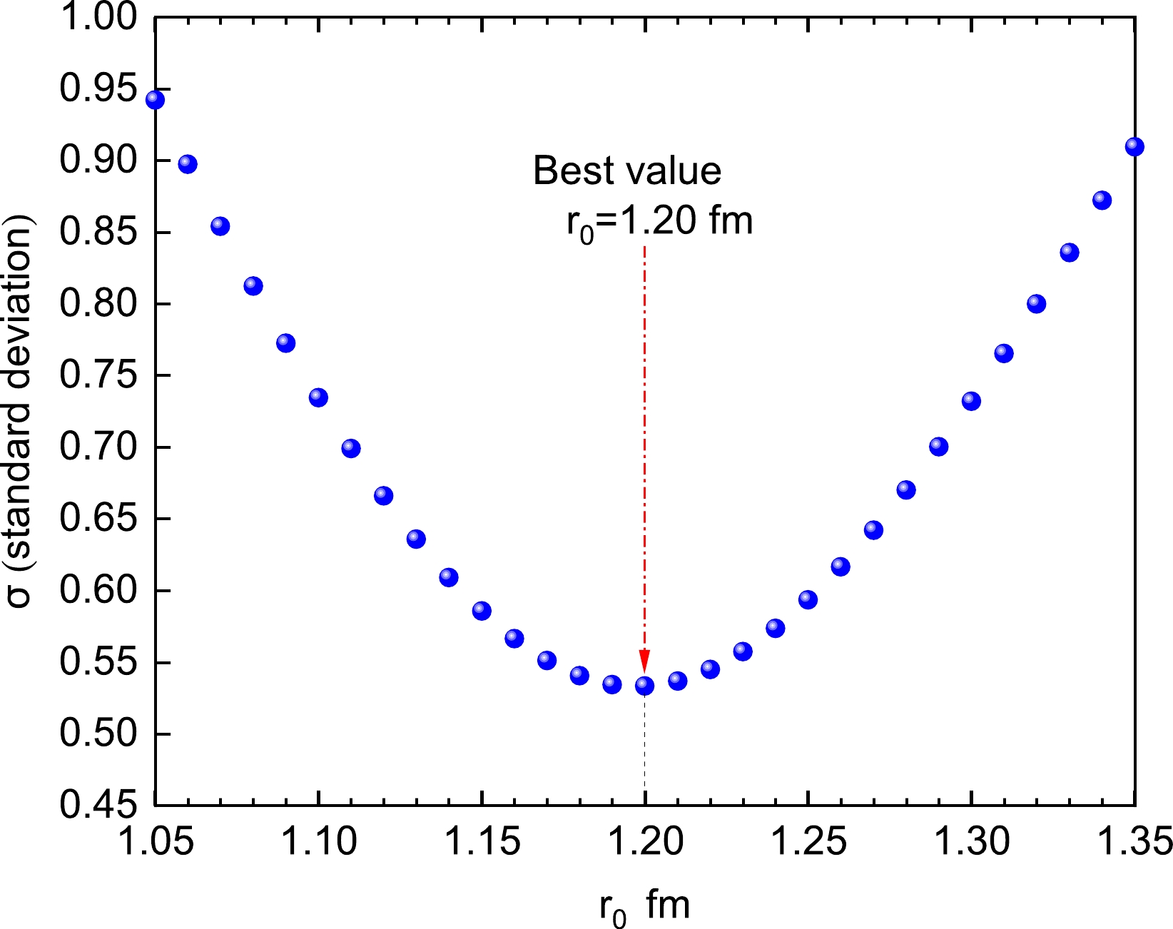

Figure 2.(color online) Relevance between the standard deviationσand the value of the parameter $ r_0 $ .

In the following, within the framework of the D-GLM, we systematically investigate the half-lives of 45 deformed proton emitters. For comparison, the calculated results obtained by the Gamow-like model proposed by Xiaoet al.[70] (GLM-Xiao), the universal decay law for proton emission (UDLP) [71], and the new Geiger-Nuttall law (NG-N) [72] are also presented.

The UDLP was proposed by Qiet al.[71] for investigating proton radioactivity, which can be expressed as

where the adjustable parameters are $a=0.386,~ b=-0.502, c=-17.8,$ and $ d=2.386 $ , respectively. The middle parameters are $ \chi^{\prime}=Z_pZ_d\sqrt{\frac{A_pA_d}{(A_p+A_d)Q_p}} $ and $\rho^{\prime}= \sqrt{\frac{Z_pZ_dA_pA_d(A_p^{1/3}+A_d^{1/3})}{A_p+A_d}}$ .

The NG-N proposed by Chenet al.[72] is a two-parameter empirical formula. It can be expressed as

where the two parameters $ a=0.843 $ and $ b=-27.194 $ were obtained by fitting 44 experimental data of the proton radioactivity half-lives.

All the specific calculated half-lives are presented in logarithmic form inTable 1. In this table, the first five columns denote the proton emitters, proton emission released energy $ Q_p $ , spin and parity transition, angular momentumltaken away by the emitted proton, and spectroscopic factor $ S_p $ , respectively. The values of $ S_p $ are derived from the relativistic mean field theory (RMF) with the Bardeen-Cooper-Schriffer (BCS) theory [6] except those for¹⁰⁸I,¹⁴⁴Tm,¹⁵⁹Re^m,¹⁷⁰Au,¹⁷⁰Au^m, and¹⁷⁶Tl, which are taken from Ref. [53]. The correlative nuclear deformation parameters are taken from Ref. [64]. The last five columns denote the experimental proton emission half-lives and the theoretical ones calculated using the D-GLM, GLM-Xiao, UDLP, and NG-N, respectively. It is worth noting that the results obtained with our model are basically consistent with the experimental data.

Nucleus $ ^{A}Z $	$ Q_p $ /MeV	$ j^{\pi}\rightarrow j_d^{\pi} $	l	$ S_p $	$ {\rm{log}}_{10}{T}_{1/2} $ (s)
					Exp	D-GLM	GLM-Xiao [70]	UDLP [71]	NG-N [72]
108I	0.610	$ (1^+)\#\rightarrow 5/2^+\# $	2	0.089	0.723	0.578		–0.019	0.829
109I	0.829	$ (3/2^+)\rightarrow 0^+ $	2	0.435	–4.032	–4.168	–5.138	–3.671	–3.157
112Cs	0.820	$ 1^+\#\rightarrow 5/2^+\# $	2	0.464	–3.310	–3.349	–3.228	–2.923	–2.362
113Cs	0.981	$ (3/2^+)\rightarrow 0^+ $	2	0.446	–4.771	–5.525	–5.338	–4.899	–4.490
117La	0.831	$ (3/2^+)\rightarrow 0^+ $	2	0.183	–1.664	–2.461	–2.757	–2.459	–1.857
Continued on next page

Table 1.Comparison of experimental proton emission half-lives with the calculated ones by using different theoretical models and/or formulae. The symbolmrepresents the first isomeric state. The experimental proton emission half-lives, spin, and parity are taken from Ref. [7]. The released energies are given by Eq. (7) with the exception of the $ Q_p $ value for¹³⁰Eu,¹⁵⁹Re,¹⁶¹Re^m,¹⁶⁴Ir, and¹⁷⁷Tl^m, which are taken from Refs. [9,73]. The values of $ S_p $ are derived from Ref. [6] except those for¹⁰⁸I,¹⁴⁴Tm,¹⁵⁹Re^m,¹⁷⁰Au,¹⁷⁰Au^m, and¹⁷⁶Tl, which are taken from Ref. [53]. The correlative nuclear deformation parameters are taken from Ref. [64].

Furthermore, for a more intuitive comparison of the experimental half-lives with the calculated ones, the deviations between the experimental proton emission half-lives and the calculated ones obtained using the above four models and/or formula e in logarithmic form are plotted inFig. 3. It can be clearly observed that the majority of deviations are within $ \pm 1 $ on the whole, which indicates that the present estimates for the proton emission half-lives using the D-GLM are adequately credible. However, for some proton emitters, the calculated half-lives with the D-GLM differ from the experimental ones by approximately one order of magnitude, corresponding to the well deformed cases of¹¹⁷La,¹²¹Pr,¹³⁵Tb, and¹⁴¹Ho. Seeking the reasons why such a large deviation occurs is a vital topic. It is well known that the calculated results are sensitive to the released energy $ Q_p $ and the angular momentuml. Consequently, the first possible reason is that the deviation between the experimental and calculated values for the above four cases is due to uncertainties in the measurements of the $ Q_p $ values. Thus, further theoretical investigation and measurements with high accuracy are required. In addition, for¹¹⁷La,¹²¹Pr,¹³⁵Tb, and¹⁴¹Ho, the proton emission half-lives in logarithmic form calculated by the D-GLM versus the $ Q_p $ in the different cases oflare presented inFig. 4. From this figure, we can found that the half-lives increase by one order of magnitude or more for each increase in angular momentum when the values of $ Q_p $ are the same and $ l>2 $ . Taking¹¹⁷La as an example, the half-lives can reproduce the experimental data well for $ l=3 $ rather than for $ l=2 $ . In the same way, for the nuclei¹²¹Pr,¹³⁵Tb, and¹⁴¹Ho, the experimental data are perfectly fitted with the values ofltaken as 3, 4, and 4, respectively. The values oflhave a higher consistency with the analytical results of Chenget al.[74], which means that the orbital angular momenta of¹¹⁷La,¹²¹Pr,¹³⁵Tb, and¹⁴¹Ho may be 3, 3, 4, and 4, respectively. Therefore, the second reason for the large deviations may be that the values oflare uncertain.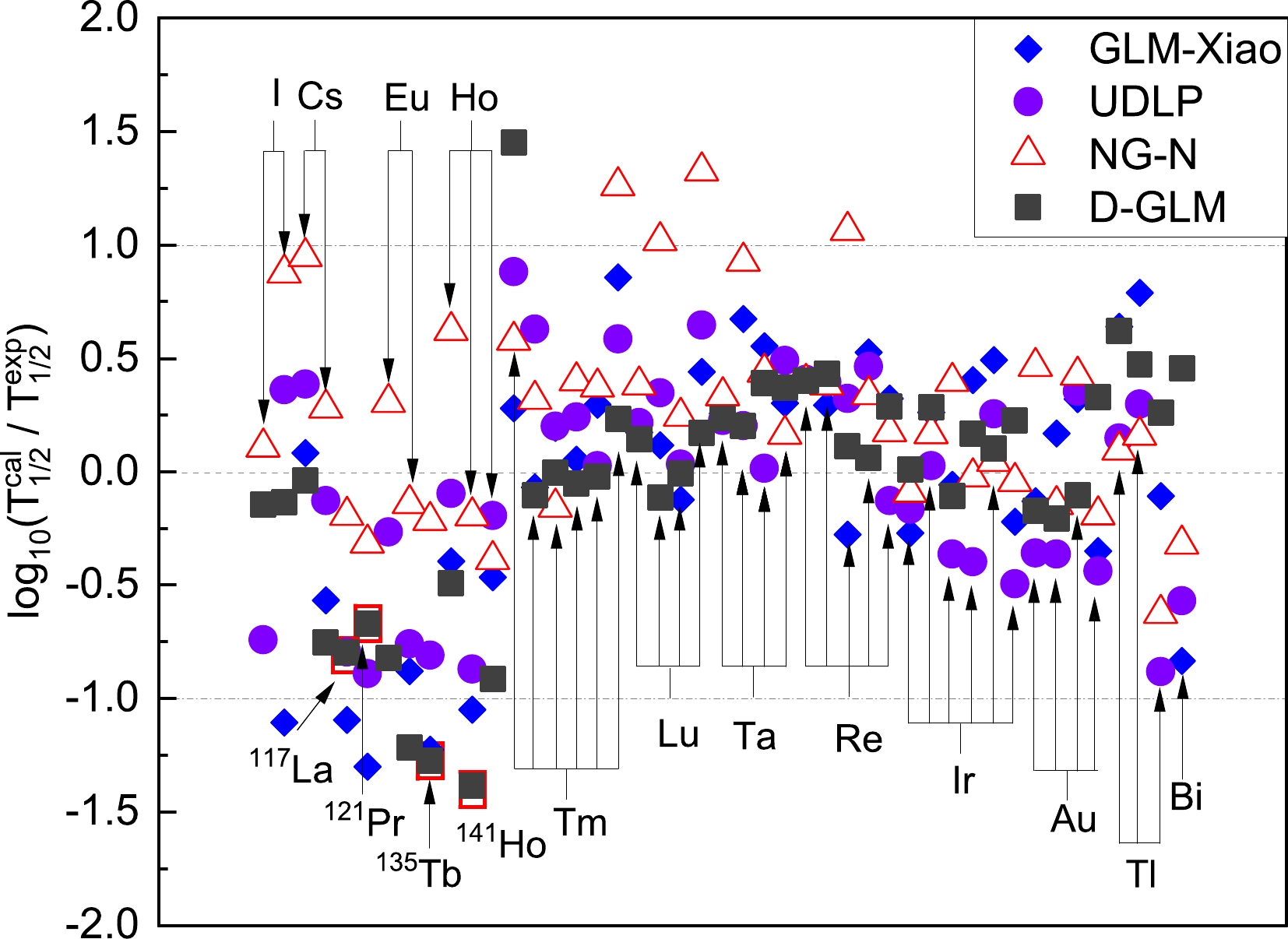

Figure 3.(color online) Deviations between the experimental proton emission half-lives and the calculated ones in logarithmic form for deformed nuclei. The blue rhombuses, purple circles, red triangles, and black squares correspond to the deviations determined by applying the GLM-Xiao, UDLP, NG-N, and D-GLM, respectively.

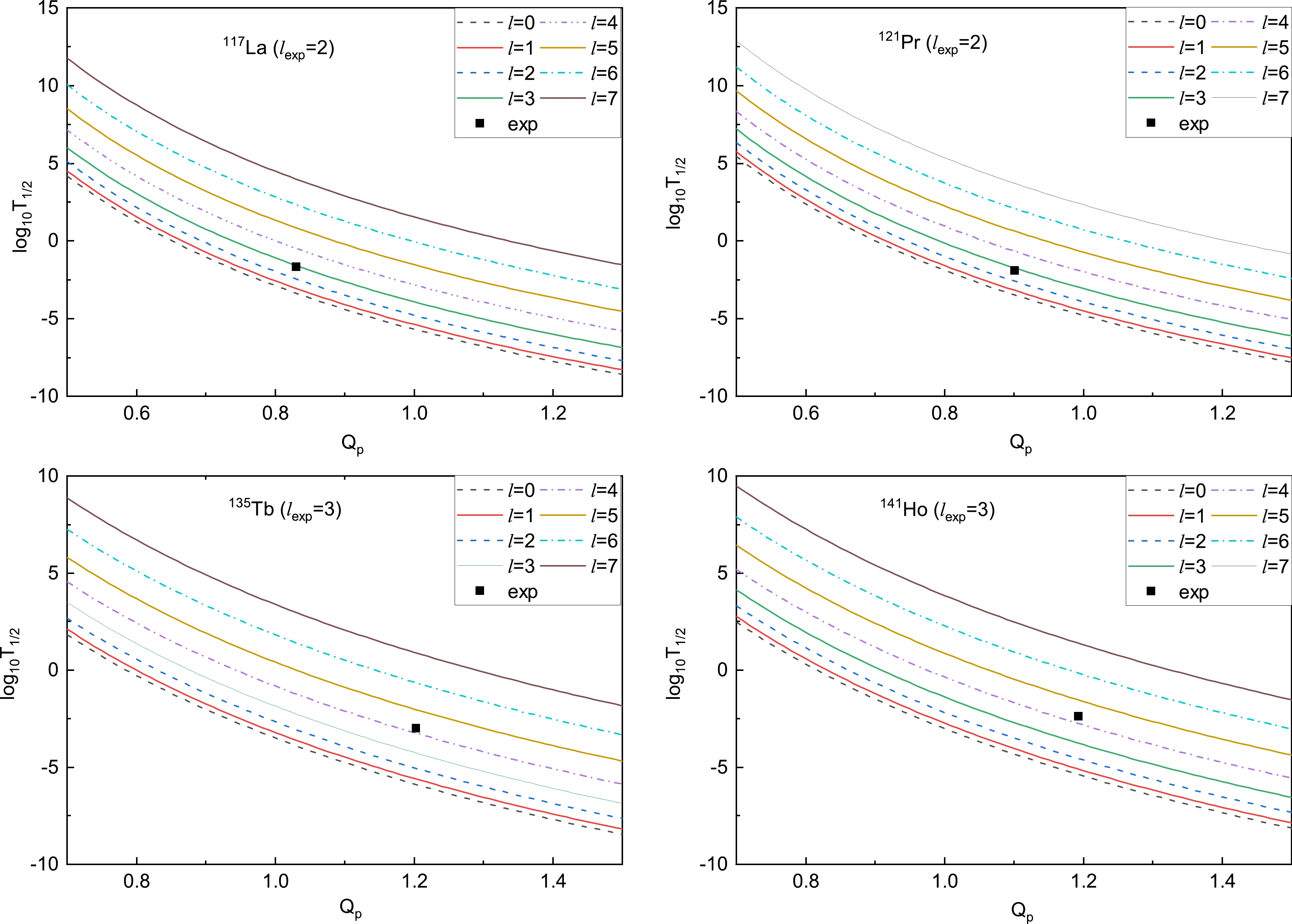
Figure 4.(color online) $ {\rm{log}}_{10}T_{1/2} $ values as functions of $ Q_p $ for¹¹⁷La,¹²¹Pr,¹³⁵Tb, and¹⁴¹Ho whenlis taken with different values.

To further verify the rationality of this conclusion, using the D-GLM, UDLP, Coulomb and proximity potential model (CPPM) [75], and unified fission model (UFM) [41], the proton emission half-lives are calculated while thelof¹¹⁷La,¹²¹Pr,¹³⁵Tb, and¹⁴¹Ho are changed to 3, 3, 4, and 4. The detailed results are presented inTable 2. From this table, we can observe that the calculated results accurately match the experimental data. Moreover, the logarithmic form of the experimental proton emission half-lives and the values calculated using the four methods mentioned above are plotted inFig. 5. The calculated results for¹¹⁷La,¹²¹Pr,¹³⁵Tb, and¹⁴¹Ho with the angular momentuml= 2, 2, 3, 3 andl= 3, 3, 4, 4 are presented inFig. 5(a) andFig. 5(b), respectively. We note that the calculated results obtained by the D-GLM, CPPM, UFM, and UDLP more accurately reflect the experimental data after the values oflare changed. The values oflmay provide a reference for future research.

Nucleus	l	$ {\rm{log}}_{10}{T}_{1/2} $ (s)
		Exp	D-GLM	CPPM [75]	UFM	UDLP [71]
117La	3	–1.664	–1.591	–1.587	–1.785	–1.667
121Pr	3	–1.921	–1.742	–2.007	–2.158	–2.036
135Tb	4	–2.996	–3.252	–2.948	–2.844	–2.837
141Ho	4	–2.387	–2.760	–2.322	–2.214	–2.310

Table 2.Calculated results of the proton emission half-lives for deformed nuclei when thelvalues of¹¹⁷La,¹²¹Pr,¹³⁵Tb, and¹⁴¹Ho are taken as 3, 3, 4, and 4.

Figure 5.(color online) Comparison of the D-GLM and UDLP results with the experimental data for proton emitter of¹¹⁷La,¹²¹Pr,¹³⁵Tb and¹⁴¹Ho forl= 2, 2, 3, 3 $ (a) $ and forl= 3, 3, 4, 4 $ (b) $ , respectively.

To globally comprehend the agreement between the experimental and calculated values, we calculate the standard deviations obtained by the D-GLM, UDLP, and NG-N, which are denoted as $ \sigma_{\rm{D-GLM}} $ , $ \sigma_{\rm{UDLP}} $ , and $ \sigma_{\rm{NG-N}} $ . As listed inTable 3, $ \sigma_{\rm{D-GLM}}=0.533 $ , $ \sigma_{{\rm{GLM-Xiao}}}=0.601 $ , $ \sigma_{\rm{UDLP}}=0.471 $ , and $ \sigma_{\rm{NG-N}}=0.515 $ . These results demonstrate that the proton emission half-lives calculated by the D-GLM have high accuracy.

In conclusion, we present a systematic study of the proton emission half-lives for 45 deformed proton emitters based on the D-GLM, which contains the deformed effect of Coulomb potential for the daughter nucleus. The proposed model contains only one adjustable parameter, that is, the effective nuclear radius constant, which is obtained by fitting 45 experimental data of the proton emission half-lives and is determined to be $ r_0=1.20 $ fm. We found that the calculated results could reproduce the experimental data well. Moreover, the relevance between the half-lives andlfor¹¹⁷La,¹²¹Pr,¹³⁵Tb, and¹⁴¹Ho was investigated, and the corresponding possible reference values were proposed:l= 3, 3, 4, 4. Future theoretical and experimental research could benefit from the useful knowledge that this work may offer.