


 Abstract
 HTML
HTML Reference
 Related
 PDF
PDF




-
Bmeson physics is an important and popular area of particle physics because of continuous impetus from experimental and theoretical efforts and pursuits. With the running of the Belle-II and LHCb experiments, an increasing number ofBmeson events will be accumulated, with an expected goal integrated luminosity of
$50\ \rm ab^{-1}$ by the Belle-II detector at the$ e^{+}e^{-} $ SuperKEKB collider [1] and approximately$300\ \rm fb^{-1}$ by the LHCb detector at the future High Luminosity LHC (HL-LHC) hadron collider [2]. More than$ 10^{11} B_{u,d} $ mesons are expected to become available at the future CEPC [3] and FCC-ee [4] experiments based on approximately$ 10^{12} Z^{0} $ boson decays with a branching ratio$ {\cal B}(Z^{0}{\to}b\bar{b})\, {\approx} 15.12 $ % [5] and a fragmentation fraction$ f(b{\to}B_{u}) {\approx} f(b{\to}B_{d}) \, {\approx} 41.8 $ % [6]. With the gradual improvement of data processing technology, besides numerous new and unforeseen phenomena, higher precision measurements ofBmeson weak decays will be achieved. The experimental study ofBmeson decays is stepping into a golden age of big data and high precision. Higher requirements have been placed on the accuracy of theoretical calculations forBmeson decays, which is the fundamental premise behind rigorous testing of the standard model (SM) of elementary particles, finding a solution to the discrepancies between data and theoretical expectations, and searching for new physics beyond the SM.Owing to an inadequate understanding of the dynamic mechanisms of hadronization and quantum chromodynamics (QCD) behavior at low energy scales, the main uncertainties on various theoretical estimations forBmeson decays arise from the hadronic matrix elements (HMEs) describing the transition from the involved quarks to hadrons. The calculation of nonleptonicBmeson decays is especially complex because both the initial and final states are hadrons. Additionally, nonleptonicBdecay modes are rich, and the study of these is interesting and significant. The measurement of nonleptonicBmeson decays has been providing abundant information and various constraints on the SM, for example, the angles and sides of the commonly termed unitarity triangle,
$ V_{ud}V_{ub}^{\ast} + V_{cd}V_{cb}^{\ast} + V_{td}V_{tb}^{\ast} = 0 $ , arising from the Cabibbo-Kobayashi-Maskawa (CKM) matrix [7,8]. The method of dealing with HMEs as reasonably and reliably as possible is now a central and urgent issue in the theoretical calculation of nonleptonicBmeson decays.Based on the widely used Lepage-Brodsky procedure for exclusive processes with a large momentum transfer between hadrons [9] and the power counting rules in heavy quark limits, several attractive QCD-inspired methods, such as the perturbative QCD (PQCD) approach [10–16], QCD factorization (QCDF) approach [17–26], and soft and collinear effective theory [27–34], have been fully developed to evaluate HMEs for nonleptonicBmeson decays, where HMEs are phenomenologically expressed as the convolution integral of the scattering amplitudes at the quark level and wave functions (WFs) (or distribution amplitudes (DAs)) at the hadronic level. The calculation accuracy of HMEs may be improved via the following two aspects together: The first is the scattering amplitudes, and the second is the hadronic WFs or DAs. Owing to the asymptotic freedom of QCD, the scattering amplitudes describing hard interactions among quarks are calculable, in principle, order by order with the perturbative quantum field theory. The higher order radiative corrections to HMEs are necessary and important for approaching the true values, reducing the dependence of theoretical results on the renormalization scale, obtaining strong phases closely related to the
$C P$ violation, verifying models, and perfecting methods. In recent years, the next-to-next-to-leading order (NNLO) corrections to HMEs have become available and have shown a large model sensitivity to the hadronic distribution amplitudes, for example, in Refs. [35–39]. The influences of WFs on HMEs are also significant; however, they have attracted relatively insufficient attention compared with the scattering amplitudes. There are numerous studies on nonleptonicBdecays using the PQCD approach, which show that the theoretical uncertainties mainly originate from the parameters of the WFs or DAs, for example, in Refs. [40–55], and the actual contributions from the higher twist (for example, twist-3) DAs to the hadronic transition form factors are as important as those from the leading twist (twist-2) DAs [42–47] and those from the next-to-leading order (NLO) QCD radiative corrections to the scattering amplitudes [41,46]. It has already been recognized from the numerical perspective that the effects from the higher twist hadronic DAs are considerably large rather than formally power suppressed.In our recent study [41],
$ B {\to} PP $ decays were systemically reinvestigated using the PQCD approach by considering contributions fromBmesonic subleading twist WFs and the updated DAs of the final pseudoscalar mesons. It was found that the contribution from theBmesonic WFs$ {\phi}_{B2} $ , which are usually paid less attention in calculations, have certain influences over HMEs and branching ratios and are comparable with those from the NLO corrections. In this work, a comprehensive study of the effects of the WFs$ {\phi}_{B2} $ and updated DAs of final states using the PQCD approach is extended to charmless$ B {\to} PV $ decays to match the precision improvement of theoretical and experimental results, whereVdenotes the ground$S U(3)$ vector mesons. Because of our inadequate understanding of the flavor mixing and possible glueball components, the final states of$ {\eta} $ and$ {\eta}^{\prime} $ mesons are not currently considered here, that is,$ P = {\pi} $ andK.This paper is organized as follows. In Section II, the theoretical framework is briefly described. Definitions of kinematic variables and expressions for the WFs involved are presented in Sections III and IV, respectively. The contributions from different twist WFs to the form factors of
$ B {\to} PV $ decays are quantitatively analyzed in Section V. In Section VI, the branching ratios and$C P$ asymmetries of the$ B {\to} PV $ decays are reevaluated by taking theBmesonic WFs$ {\phi}_{B2} $ into consideration. We conclude with a summary in Section VII. The decay amplitudes and amplitude building blocks for the$ B {\to} PV $ decays are displayed in Appendices A and B, respectively. -
It is widely accepted that charmless nonleptonic
$ B {\to} PV $ decays are predominantly induced by heavybquark weak decays within the SM, that is,$ b {\to} W^{{\ast}-} + u $ . There are at least three energy scales, the mass of the$ W^{\pm} $ gauge boson$ m_{W} $ , the mass of thebquark$ m_{b} $ , and the QCD characteristic scale$ {\Lambda}_{\rm QCD} $ , with the hierarchical relationship$ m_{W} {\gg} m_{b} {\gg} {\Lambda}_{\rm QCD} $ and each energy scale corresponding to a different interaction dynamic. Based on the operator product expansion and renormalization group (RG) method, the effective Hamiltonian in charge of charmless$ B {\to} PV $ decays can be factorized by the renormalization scale$ {\mu} $ into three parts, the Wilson coefficients$ C_{i} $ , four-quark operators$ Q_{i} $ , and$ {\mu} $ -independent couplings of weak interactions, including the Fermi constant$G_{\rm F} {\approx} 1.166{\times}10^{-5} {\rm GeV}^{-2}$ [5] and CKM factors, and expressed as [56]$ {\cal H}_{\rm eff}\, =\, \frac{G_{\rm F}}{\sqrt{2}}\, \sum\limits_{q=d,s} \Bigg\{ V_{ub}\,V_{uq}^{\ast} \sum\limits_{i=1}^{2}C_{i}\,Q_{i} - V_{tb}\,V_{tq}^{\ast} \sum\limits_{j=3}^{10}C_{j}\,O_{j} \Bigg\} +{\rm h.c.} $

(1) With the phenomenological Wolfenstein parametrization and up to
$ {\cal O}({\lambda}^{8}) $ , the CKM factors involved are expressed as$ V_{ub}\,V_{ud}^{\ast} = A\,{\lambda}^{3}\,({\rho}-{\rm i}\,{\eta})\left( 1-\frac{1}{2}\lambda^2-\frac{1}{8}\lambda^4 \right)+{\cal O}(\lambda^8), $

(2) $ V_{tb}\,V_{td}^{\ast} = A\,{\lambda}^{3} +A^{3}\,{\lambda}^{7}\,\left({\rho}-{\rm i}\,{\eta}-\frac{1}{2}\right) -V_{ub}\,V_{ud}^{\ast} +{\cal O}({\lambda}^{8}) , $

(3) $ V_{ub}\,V_{us}^{\ast} = A\,{\lambda}^{4}\,({\rho}-{\rm i}\,{\eta}) +{\cal O}({\lambda}^{8}) , $

(4) $ \begin{aligned}[b] V_{tb}\,V_{ts}^{\ast} =& -A\,{\lambda}^{2}\,\left(1-\frac{1}{2}\,{\lambda}^{2}-\frac{1}{8}\,{\lambda}^{4}\right) +\frac{1}{2}\,A^{3}\,{\lambda}^{6} -V_{ub}\,V_{us}^{\ast} +{\cal O}({\lambda}^{8}) , \end{aligned} $

(5) whereA,
$ {\lambda} $ ,$ {\rho} $ , and$ {\eta} $ are the Wolfenstein parameters; their latest fitted values can be found in Ref. [5]. The Wilson coefficients$ C_{i} $ summarize physical contributions above the energy scale$ {\mu} $ and are computable using the RG-assisted perturbative theory. Their explicit expressions, including the NLO corrections, can be found in Ref. [56]. The local four-quark operators are defined as follows:$ Q_{1} \, =\, \big[\, \bar{u}_{\alpha}\,{\gamma}_{\mu}\,(1-{\gamma}_{5})\,b_{\alpha} \,\big]\ \big[\, \bar{q}_{\beta}\,{\gamma}^{\mu}\,(1-{\gamma}_{5})\,u_{\beta} \,\big] , $

(6) $ Q_{2} \, =\, \big[\, \bar{u}_{\alpha}\,{\gamma}_{\mu}\,(1-{\gamma}_{5})\,b_{\beta} \,\big]\ \big[\, \bar{q}_{\beta}\,{\gamma}^{\mu}\,(1-{\gamma}_{5})\,u_{\alpha} \,\big] , $

(7) $ Q_{3} \, =\, \sum\limits_{q^{\prime}}\, \big[\, \bar{q}_{\alpha}\,{\gamma}_{\mu}\,(1-{\gamma}_{5})\,b_{\alpha} \,\big]\ \big[\, \bar{q}^{\prime}_{\beta}\,{\gamma}^{\mu}\,(1-{\gamma}_{5})\,q^{\prime}_{\beta} \,\big] , $

(8) $ Q_{4} \, =\, \sum\limits_{q^{\prime}}\, \big[\, \bar{q}_{\alpha}\,{\gamma}_{\mu}\,(1-{\gamma}_{5})\,b_{\beta} \,\big]\ \big[\, \bar{q}^{\prime}_{\beta}\,{\gamma}^{\mu}\,(1-{\gamma}_{5})\,q^{\prime}_{\alpha} \,\big] , $

(9) $ Q_{5} \, =\, \sum\limits_{q^{\prime}} \, \big[\, \bar{q}_{\alpha}\,{\gamma}_{\mu}\,(1-{\gamma}_{5})\,b_{\alpha} \,\big]\ \big[\, \bar{q}^{\prime}_{\beta}\,{\gamma}^{\mu}\,(1+{\gamma}_{5})\,q^{\prime}_{\beta} \,\big] , $

(10) $ Q_{6} \, =\, \sum\limits_{q^{\prime}} \big[\, \bar{q}_{\alpha}\,{\gamma}_{\mu}\,(1-{\gamma}_{5})\,b_{\beta} \,\big]\ \big[\, \bar{q}^{\prime}_{\beta}\,{\gamma}^{\mu}\,(1+{\gamma}_{5})\,q^{\prime}_{\alpha} \,\big] , $

(11) $ Q_{7} \, =\, \sum\limits_{q^{\prime}}\,\frac{3}{2}\,Q_{q^{\prime}}\, \big[\, \bar{q}_{\alpha}\,{\gamma}_{\mu}\,(1-{\gamma}_{5})\,b_{\alpha} \,\big]\ \big[\, \bar{q}^{\prime}_{\beta}\,{\gamma}^{\mu}\,(1+{\gamma}_{5})\,q^{\prime}_{\beta} \,\big] , $

(12) $ Q_{8} \, =\, \sum\limits_{q^{\prime}}\,\frac{3}{2}\,Q_{q^{\prime}}\, \big[\, \bar{q}_{\alpha}\,{\gamma}_{\mu}\,(1-{\gamma}_{5})\,b_{\beta} \,\big]\ \big[\, \bar{q}^{\prime}_{\beta}\,{\gamma}^{\mu}\,(1+{\gamma}_{5})\,q^{\prime}_{\alpha} \,\big] , $

(13) $ Q_{9} \, =\, \sum\limits_{q^{\prime}}\,\frac{3}{2}\,Q_{q^{\prime}}\, \big[\, \bar{q}_{\alpha}\,{\gamma}_{\mu}\,(1-{\gamma}_{5})\,b_{\alpha} \,\big]\ \big[\, \bar{q}^{\prime}_{\beta}\,{\gamma}^{\mu}\,(1-{\gamma}_{5})\,q^{\prime}_{\beta} \,\big] , $

(14) $ Q_{10} = \sum\limits_{q^{\prime}}\,\frac{3}{2}\,Q_{q^{\prime}} \big[ \bar{q}_{\alpha}\,{\gamma}_{\mu}\,(1-{\gamma}_{5})\,b_{\beta} \,\big]\ \big[\, \bar{q}^{\prime}_{\beta}\,{\gamma}^{\mu}\,(1-{\gamma}_{5})\,q^{\prime}_{\alpha} \big] , $

(15) where
$ {\alpha} $ and$ {\beta} $ are the color indices,$ q^{\prime} {\in} $ $\{ u $ ,d,c,s,$ b\} $ , and$ Q_{q^{\prime}} $ is the electric charge of quark$ q^{\prime} $ in the unit of$ {\vert}e{\vert} $ . The physical contributions below the energy scale$ {\mu} $ are contained in the HMEs$ {\langle}Q_{i}{\rangle} = {\langle}PV{\vert}Q_{i}{\vert}B{\rangle} $ , which are the focus of the current theoretical calculation.The various treatments on HMEs depend on the different phenomenological approaches corresponding to the understanding of the perturbative and nonperturbative contributions. The joint effort of the transverse momentum for quarks and the Sudakov factors for all participant WFs is considered within the PQCD approach to settle the soft endpoint contributions from the collinear approximation. The master formula for HMEs with the PQCD approach is generally written as
$ \begin{aligned}[b] {\langle}PV{\vert}Q_{i}{\vert}B{\rangle} {\propto}& {\int} {\rm d}x_{1} {\rm d}x_{2} {\rm d}x_{3} {\rm d}b_{1}{\rm d}b_{2}{\rm d}b_{3}\, H_{i}(t_{i},x_{1},b_{1},x_{2},b_{2},x_{3},b_{3}) \\ & \times {\Phi}_{B}(x_{1},b_{1})\,{\rm e}^{-S_{B}}\, {\Phi}_{P}(x_{2},b_{2})\,{\rm e}^{-S_{P}}\, {\Phi}_{V}(x_{3},b_{3})\,{\rm e}^{-S_{V}} , \end{aligned} $

(16) where
$ b_{i} $ is the conjugate variable of the transverse momentum$ \vec{k}_{i{\perp}} $ of the valence quarks,$ H_{i} $ is the scattering amplitudes for hard gluon exchange interactions among quarks, and${\rm e}^{-S_{i}}$ is the Sudakov factor. Other variables and inputs are described below. -
It is usually assumed that in the heavy quark limit, light quarks rapidly move away from thebquark decaying point at near the speed of light. Moreover, light cone variables are generally used in expressions. The relations between the four-dimensional space-time coordinates
$ x^{\mu} = $ ($ x^{0} $ ,$ x^{1} $ ,$ x^{2} $ ,$ x^{3} $ )$ = $ (t,x,y,z) and the light-cone coordinates$ x^{\mu} = $ ($ x^{+} $ ,$ x^{-} $ ,$ \vec{x}_{\perp} $ ) are defined as$ x^{\pm} = (x^{0}{\pm}x^{3})/\sqrt{2} $ and$ \vec{x}_{\perp} = $ ($ x^{1} $ ,$ x^{2} $ ). The light cone planes correspond to$ x^{\pm} = 0 $ . The scalar product of any two vectors is given by$a{\cdot}b = a_{\mu}b^{\mu} = a^{+}b^{-} + a^{-}b^{+} - \vec{a}_{\perp}{\cdot}\vec{b}_{\perp}$ .In the rest frame of theBmeson, the light cone kinematic variables are defined as
$ p_{B}\, =\, p_{1}\, =\, \frac{m_{B}}{\sqrt{2}}(1,1,0) , $

(17) $ p_{P}\, =\, p_{2}\, =\, \frac{m_{B}}{\sqrt{2}}(0,1-r_{V}^{2},0) , $

(18) $ p_{V}\, =\, p_{3}\, =\, \frac{m_{B}}{\sqrt{2}}(1,r_{V}^{2},0) , $

(19) $ e^{\parallel}_{V}\, =\, \frac{p_{V}}{m_{V}}- \frac{m_{V}}{p_{V}{\cdot}n_-}n_- , $

(20) $ k_{1}\, =\, x_{1}\,p_{1}+(0,0,\vec{k}_{1{\perp}}) , $

(21) $ k_{2}\, =\, \frac{m_{B}}{\sqrt{2}}(0,x_{2},\vec{k}_{2{\perp}}) , $

(22) $ k_{3}\, =\, \frac{m_{B}}{\sqrt{2}}(x_{3},0,\vec{k}_{3{\perp}}) , $

(23) where the mass ratio
$ r_{V} = m_{V}/m_{B} $ ,$ e^{\parallel}_{V} $ is the longitudinal polarization vector, and the variables$ x_{1} $ and$ \vec{k}_{1{\perp}} $ are the longitudinal momentum fraction and transverse momentum of the light quark in theBmeson, respectively. The variables$ x_{i} $ and$ \vec{k}_{i{\perp}} $ for$ i = 2 $ and$ 3 $ are the longitudinal momentum fractions and transverse momentum of the antiquarks in the final pseudoscalar and vector mesons, respectively. -
Bmesonic WFs are generally defined as [41–43,57,58]
$ \begin{aligned}[b] & {\langle}\,0\,{\vert}\, \bar{q}_{\alpha}(z)\,b_{\beta}(0)\,{\vert}\, \overline{B}(p_{1})\,{\rangle} \\ =& +\frac{\rm i}{4}f_{B} {\int} {\rm d}^{4}k {\rm e}^{-{\rm i}\,k_{1}{\cdot}z}\, \Bigg\{ \big( \not {p}_{1}+m_{B}\big) {\gamma}_{5}\, \Bigg[\,\frac{\not {n}_-}{\sqrt{2}}\,{\phi}_{B}^+ +\frac{\not {n}_+}{\sqrt{2}}\,{\phi}_{B}^- \Bigg] \Bigg\}_{{\beta}{\alpha}} \\ =& -\frac{\rm i}{4}\,f_{B}\,{\int} {\rm d}^{4}k{\rm e}^{-{\rm i}\,k_{1}{\cdot}z} \Bigg\{ \big( \not {p}_{1}+m_{B}\big) {\gamma}_{5} \Bigg[{\phi}^++\frac{\not {n}_+}{\sqrt{2}}\,\big( {\phi}_{B}^+-{\phi}_{B}^- \big) \Bigg] \Bigg\}_{{\beta}{\alpha}} \\ =& -\frac{\rm i}{4}\,f_{B}\,{\int} {\rm d}^{4}k {\rm e}^{-{\rm i}\,k_{1}{\cdot}z} \Bigg\{ \big( \not {p}_{1}+m_{B}\big) {\gamma}_{5} \Bigg({\phi}_{B1}+\frac{\not {n}_+}{\sqrt{2}}\, {\phi}_{B2} \Bigg) \Bigg\}_{{\beta}{\alpha}} , \end{aligned} $

(24) where
$ f_{B} $ is the decay constant. The coordinatezof the light quark and the vectors$ n_{+} = $ ($ 1 $ ,$ 0 $ ,$ \vec{0} $ ) and$ n_{-} = $ ($ 0 $ ,$ 1 $ ,$ \vec{0} $ ) are on the light cone, that is,$ z^{2} = 0 $ and$ n_{\pm}^{2} = 0 $ . The scalar functions$ {\phi}_{B}^{+} $ and$ {\phi}_{B}^{-} $ are the leading and subleading twist WFs, respectively.$ {\phi}_{B}^{+} $ and$ {\phi}_{B}^{-} $ have different asymptotic behaviors as the longitudinal momentum fraction of the light quark$ x_{1} {\to} 0 $ . Their relations are$ {\phi}_{B}^+(x_{1}) + x_{1}\, {\phi}_{B}^{-{\prime}}(x_{1})\, =\, 0 , $

(25) $ {\phi}_{B1}\, =\, {\phi}_{B}^+ , $

(26) $ {\phi}_{B2}\, =\, {\phi}_{B}^+-{\phi}_{B}^- . $

(27) Although the expressions of
$ {\phi}_{B}^{+} $ are generally different from those of$ {\phi}_{B}^{-} $ with the equation of motion Eq. (25), an approximation of$ {\phi}_{B}^{+} = {\phi}_{B}^{-} $ is often used in phenomenological studies of nonleptonicBmeson decays, that is, only contributions from$ {\phi}_{B1} $ are considered, and those from$ {\phi}_{B2} $ are absent. However, it has been shown in Refs. [40–46] that$ {\phi}_{B2} $ is necessary to HMEs rather than a negligible factor, and its contributions to the form factors$ F_{0}^{B{\to}{\pi}} $ with the PQCD approach can even reach up to$ 30 $ % in certain cases [42,43]. Additionally, its share of the branching ratio could be as large as those from NLO corrections [41]. The possible influence of$ {\phi}_{B2} $ on$ B {\to} PV $ decays with the PQCD approach is a focus of this paper. One candidate for the most commonly used leadingBmesonic WFs$ {\phi}_{B}^{+} $ in actual calculations with the PQCD approach is expressed as [14]$ {\phi}_{B}^+(x_{1},b_{1})\, =\, N\, x_{1}^{2}\,\bar{x}_{1}^{2}\, {\exp}\Bigg\{ -\Bigg( \frac{x_{1}\,m_{B}}{\sqrt{2}\,{\omega}_{B}} \Bigg)^{2} -\frac{1}{2} {\omega}_{B}^{2}\,b_{1}^{2} \Bigg\} , $

(28) and the correspondingBmesonic WFs
$ {\phi}_{B}^{-} $ is written as [41,42]$ \begin{aligned}[b] {\phi}_{B}^-(x_{1},b_{1}) =& N\, \frac{2\,{\omega}_{B}^{4}}{m_{B}^{4}}\, {\exp}\Bigg(-\frac{1}{2} {\omega}_{B}^{2}\,b_{1}^{2} \Bigg)\,\Bigg\{ \sqrt{{\pi}}\,\frac{m_{B}}{\sqrt{2}\,{\omega}_{B}} \\&\times {\rm Erf}\Bigg( \frac{m_{B}}{\sqrt{2}\,{\omega}_{B}}, \frac{x_{1}\,m_{B}}{\sqrt{2}\,{\omega}_{B}}\Bigg) \\ & + \Bigg[1+\Bigg(\frac{m_{B}\,\bar{x}_{1}}{\sqrt{2}\,{\omega}_{B}}\Bigg)^{2}\Bigg] {\exp}\Bigg[-\Bigg(\frac{x_{1}\,m_{B}}{\sqrt{2}\,{\omega}_{B}}\Bigg)^{2} \Bigg] \\& -{\exp}\Bigg(-\frac{m_{B}^{2}}{2\,{\omega}_{B}^{2}} \Bigg) \Bigg\} , \end{aligned} $

(29) where
$ {\omega}_{B} $ is the shape parameter, and$ \bar{x}_{1} = 1 - x_{1} $ . The normalization constantNis determined by$ {\int}_{0}^{1}{\rm d}x_{1}\, {\phi}_{B}^{\pm}(x_{1},0)\, =\, 1 . $

(30) The WFs of the final states including the light pseudoscalar mesons and longitudinally polarized vector mesons are respectively defined as [59–62]
$ \begin{aligned}[b] &{\langle}\,P(p_{2})\,{\vert}\,\bar{q}_{i}(0)\,q_{j}(z)\, {\vert}\,0\,{\rangle} \\ =& -{\rm i} \frac{f_P}{4}\,{\int}_{0}^{1} {\rm d}x_{2}\, {\rm e}^{+{\rm i}\,k_{2}{\cdot}z}\, \Big\{ {\gamma}_{5}\, \Big[ \not {p}_{2}\,{\phi}_{P}^{a}+ {\mu}_{P}\,{\phi}_{P}^{p}-{\mu}_{P}\, (\not {n}_- \not {n}_+-1)\, {\phi}_{P}^{t} \Big] \Big\}_{ji} , \end{aligned} $

(31) $ \begin{aligned}[b] &{\langle}\,V(p_{3},e_{\parallel})\,{\vert}\, \bar{q}_{i}(0)\,q_{j}(z)\,{\vert}\,0\,{\rangle} \\ =& \frac{1}{4}\, {\int}_{0}^{1}{\rm d}x_{3}\, {\rm e}^{+{\rm i}\,k_{3}{\cdot}z}\, \big\{ \not {e}_{{\parallel}}\,m_{V}\,f_{V}^{\parallel}\, {\phi}_{V}^{v}\,+ \not {e}_{{\parallel}} \not {p}_{3}\, f_{V}^{\perp}\, {\phi}_{V}^{t}- m_{V}\, f_{V}^{\perp}\, {\phi}_{V}^{s} \big\}_{ji} , \end{aligned} $

(32) where
$ f_{P} $ ,$ f_{V}^{\parallel} $ , and$ f_{V}^{\perp} $ are the decay constants,$ {\phi}_{P}^{a} $ and$ {\phi}_{V}^{v} $ are the twist-2 WFs, and$ {\phi}_{P}^{p,t} $ and$ {\phi}_{V}^{t,s} $ are the twist-3 WFs. It has been previously shown that the numerical values of the form factor$ F_{0,1}^{B{\to}{\pi}} $ were highly dependent on the models for pionic WFs [42,44–46], and the contributions from the twist-3 pionic DAs to$ F_{0,1}^{B{\to}{\pi}} $ were larger than those from twist-2 pionic DAs [42,45,46]. According to the convention of Refs. [61,62], and taking the pseudoscalar$ P = K $ meson and vector$ V = K^{\ast} $ meson as an example, their DAs are written as$ {\phi}_{K}^{a}(x)\, =\, 6\,x\,\bar{x}\,\big\{ 1+a_{1}^{K}\,C_{1}^{3/2}({\xi}) +a_{2}^{K}\,C_{2}^{3/2}({\xi})\big\} , $

(33) $ \begin{aligned}[b] {\phi}_{K}^{p}(x) =& 1+3\,{\rho}_+^{K} -9\, {\rho}_-^{K}\,a_{1}^{K} +18\,{\rho}_+^{K}\,a_{2}^{K} \\ &+ \frac{3}{2}\,({\rho}_+^{K}+{\rho}_-^{K})\, (1-3\,a_{1}^{K}+6\,a_{2}^{K})\,{\ln}(x) \\ &+ \frac{3}{2}\,({\rho}_+^{K}-{\rho}_-^{K})\, (1+3\,a_{1}^{K}+6\,a_{2}^{K})\,{\ln}(\bar{x}) \\ &- (\frac{3}{2}\, {\rho}_-^{K} -\frac{27}{2}\,{\rho}_+^{K}\,a_{1}^{K} +27\,{\rho}_-^{K}\,a_{2}^{K} )\,C_{1}^{1/2}(\xi) \\ &+ ( 30\,{\eta}_{K}-3\,{\rho}_-^{K}\,a_{1}^{K} +15\, {\rho}_+^{K}\,a_{2}^{K})\,C_{2}^{1/2}(\xi) , \end{aligned} $

(34) $ \begin{aligned}[b] {\phi}_{K}^{t}(x) =& \frac{3}{2}\,({\rho}_-^{K}-3\,{\rho}_+^{K}\,a_{1}^{K} +6\,{\rho}_-^{K}\,a_{2}^{K}) \\ &- C_{1}^{1/2}(\xi)\big\{ 1+3\,{\rho}_+^{K}-12\,{\rho}_-^{K}\,a_{1}^{K} +24\,{\rho}_+^{K}\,a_{2}^{K} \\ & + \frac{3}{2}\,({\rho}_+^{K}+{\rho}_-^{K})\, (1-3\,a_{1}^{K}+6\,a_{2}^{K})\,{\ln}(x) \\ & + \frac{3}{2}\,({\rho}_+^{K}-{\rho}_-^{K})\, (1+3\,a_{1}^{K}+6\,a_{2}^{K})\, {\ln}(\bar{x}) \big\} \\ &- 3 (3\,{\rho}_+^{K}\,a_{1}^{K} -\frac{15}{2}\,{\rho}_-^{K}\,a_{2}^{K} ) C_{2}^{1/2}(\xi) , \end{aligned} $

(35) $ {\phi}_{K^{\ast}}^{v}(x) \,= \, 6\,x\,\bar{x}\, \big\{ 1 + a_{1}^{{\parallel},K^{\ast}}\,C_{1}^{3/2}(\xi) + a_{2}^{{\parallel},K^{\ast}}\,C_{2}^{3/2}(\xi) \big\} , $

(36) $ \begin{aligned}[b] {\phi}_{K^{\ast}}^{t}(x) =& 3\,{\xi}\,\big\{ C_{1}^{1/2}({\xi}) +a_{1}^{{\perp},K^{\ast}}\,C_{2}^{1/2}({\xi}) +a_{2}^{{\perp},K^{\ast}}\,C_{3}^{1/2}({\xi}) \big\} \\ &+ \frac{3}{2}\, \frac{ m_{s}+m_{q} }{ m_{K^{\ast}} }\, \frac{ f_{K^{\ast}}^{\parallel} }{ f_{K^{\ast}}^{\perp} }\, \big\{ 1 + 8\,{\xi}\,a_{1}^{{\parallel},K^{\ast}} +(21-90\,x\,\bar{x})\,a_{2}^{{\parallel},K^{\ast}} \\ & +{\xi}\,{\ln}\bar{x}\,(1+3\,a_{1}^{{\parallel},K^{\ast}} +6\,a_{2}^{{\parallel},K^{\ast}}) -{\xi}\,{\ln}x\,(1 - 3\,a_{1}^{{\parallel},K^{\ast}} + 6\,a_{2}^{{\parallel},K^{\ast}}) \big\} \\ &- \frac{3}{2}\, \frac{ m_{s}-m_{q} }{ m_{K^{\ast}} }\, \frac{ f_{K^{\ast}}^{\parallel} }{ f_{K^{\ast}}^{\perp} }\, {\xi}\, \big\{ 2 + 9\,{\xi}\,a_{1}^{{\parallel},K^{\ast}} +(22-60\,x\,\bar{x})\,a_{2}^{{\parallel},K^{\ast}} \\ & +{\ln}\bar{x}\,(1+3\,a_{1}^{{\parallel},K^{\ast}} +6\,a_{2}^{{\parallel},K^{\ast}}) +{\ln}x\,(1-3\,a_{1}^{{\parallel},K^{\ast}} +6\,a_{2}^{{\parallel},K^{\ast}}) \big\} , \end{aligned} $

(37) $ \begin{aligned}[b] {\phi}_{K^{\ast}}^{s}(x) =& - 3\,C_{1}^{1/2}({\xi}) - 3\,C_{2}^{1/2}({\xi})\,a_{1}^{{\perp},K^{\ast}} - 3\,C_{3}^{1/2}({\xi})\,a_{2}^{{\perp},K^{\ast}} \\ &- \frac{3}{2}\, \frac{ m_{s}+m_{q} }{ m_{K^{\ast}} }\, \frac{ f_{K^{\ast}}^{\parallel} }{ f_{K^{\ast}}^{\perp} }\, \big\{ C_{1}^{1/2}({\xi}) +2\,C_{2}^{1/2}({\xi})\,a_{1}^{{\parallel},K^{\ast}} \\ & + \big[ 3\,C_{3}^{1/2}({\xi}) +18\, C_{1}^{1/2}({\xi}) \big]\,a_{2}^{{\parallel},K^{\ast}} \\ & + ({\ln}\bar{x}+1)\, (1+3\,a_{1}^{{\parallel},K^{\ast}} +6\,a_{2}^{{\parallel},K^{\ast}}) \\ & - ({\ln}x+1)\, (1-3\,a_{1}^{{\parallel},K^{\ast}} +6\,a_{2}^{{\parallel},K^{\ast}}) \big\} \\ &+ \frac{3}{2}\, \frac{ m_{s}-m_{q} }{ m_{K^{\ast}} }\, \frac{ f_{K^{\ast}}^{\parallel} }{ f_{K^{\ast}}^{\perp} }\, \big\{ 9\,C_{1}^{1/2}({\xi})\,a_{1}^{{\parallel},K^{\ast}} +10\, C_{2}^{1/2}({\xi})\,a_{2}^{{\parallel},K^{\ast}} \\ & +({\ln}\bar{x}+1)\, (1+3\,a_{1}^{{\parallel},K^{\ast}} +6\,a_{2}^{{\parallel},K^{\ast}}) \\ & +({\ln}x+1)\, (1-3\,a_{1}^{{\parallel},K^{\ast}} +6\,a_{2}^{{\parallel},K^{\ast}}) \big\} , \end{aligned} $

(38) wherexis the longitudinal momentum fraction of the strange quark, and
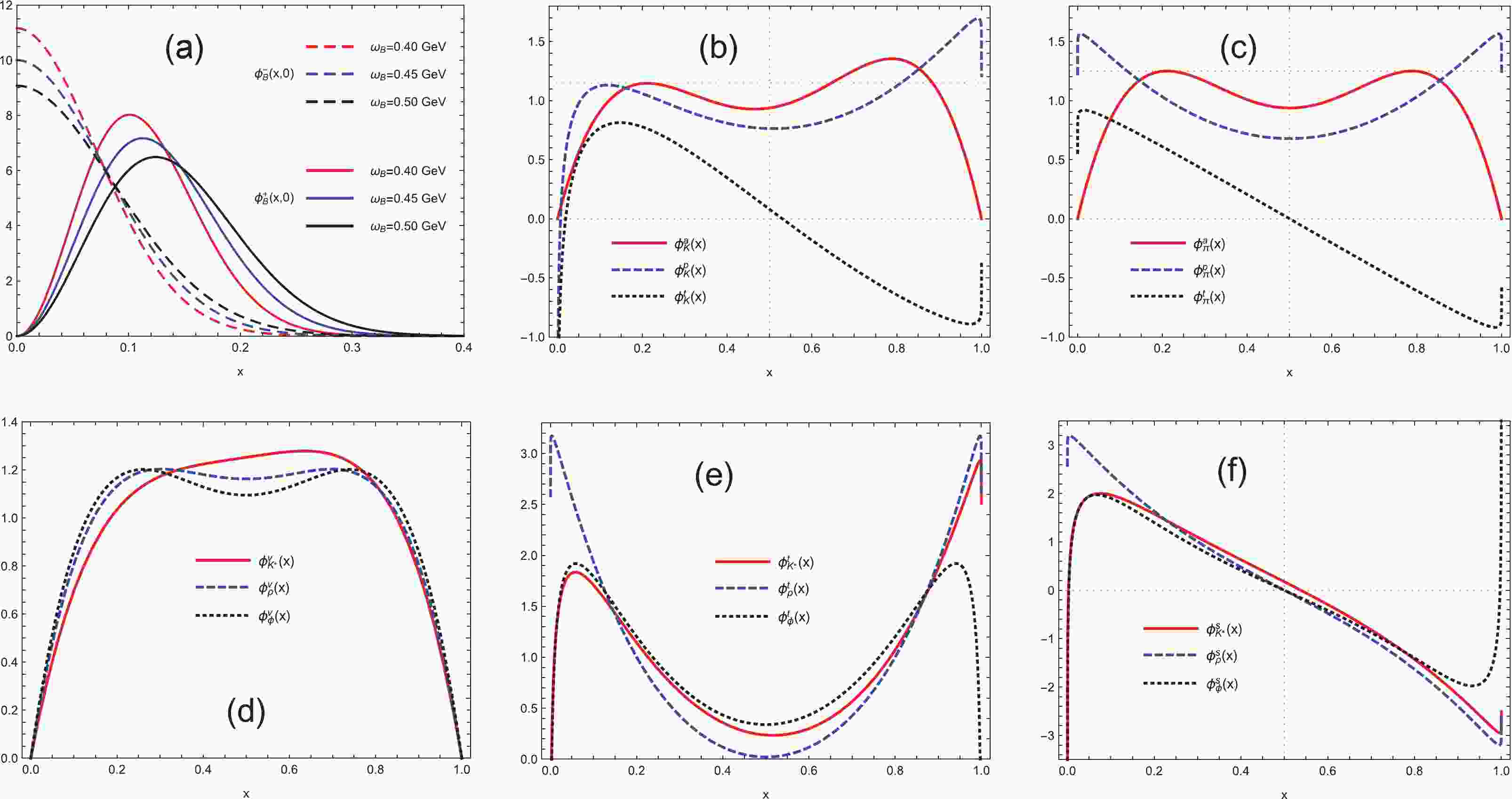
$ {\xi} = x - \bar{x} = 2\,x - 1 $ .$ C_{n}^{m} $ is the Gegenbauer polynomials.$ a_{n}^{K} $ ,$ a_{n}^{{\parallel},K^{\ast}} $ , and$ a_{n}^{{\perp},K^{\ast}} $ are the Gegenbauer moments. The dimensionless parameters${\rho}_{+}^{K} = (m_{s}+ m_{q})^{2}/m_{K}^{2}$ and$ {\rho}_{-}^{K} = (m_{s}^{2}-m_{q}^{2})/m_{K}^{2} $ [61].The shape lines of mesonic DAs with the inputs inTable 1are displayed inFig. 1. From this, the following is clear: (1) The nonzero distributions of
$ {\phi}_{B}^{\pm} $ are mainly located in the smallxregions, and$ {\phi}_{B}^{\pm} $ vanishes as$ {x} {\to} 1 $ . This fact is consistent with the intuitive expectation that the light quark shares a small longitudinal momentum fraction in theBmeson. (2) The shape lines of$ {\phi}_{B}^{-} $ differ from those of$ {\phi}_{B}^{+} $ in the smallxregions. It is particularly noticeable that the DAs$ {\phi}_{B}^{-} $ and$ {\phi}_{B}^{+} $ exhibit different endpoint behaviors at$ x = 0 $ . Thus, it is clear that${\phi}_{B2} = {\phi}_{B}^{+} - {\phi}_{B}^{-} {\ne} 0$ , and the approximation$ {\phi}_{B2} = 0 $ in previous studies might be inappropriate and insufficient. (3) The integral${\int}{\rm d}x\frac{{\phi}_{B}^{-}}{x}$ will appear in the scattering amplitudes, for example, the form factors for the transition from theBmeson to final hadrons. The value of$ {\phi}_{B}^{-} $ increases with a decrease inx, which implies that the integrals${\int}{\rm d}x\frac{{\phi}_{B}^{-}}{x}$ and${\int}{\rm d}x\frac{{\phi}_{B2}}{x}$ may be significant in the smallxregions. The potential contributions from the subleading DAs$ {\phi}_{B}^{-} $ could be greatly enhanced whenxapproaches zero and should be given due consideration in the calculation. (4) The values of$ {\phi}_{B}^{-} $ and$ {\phi}_{B2} $ are nonzero at the endpoint$ x = 0 $ ; therefore, the integral${\int}{\rm d}x\frac{{\phi}_{B2}}{x}$ will be infrared divergent at the endpoint with the collinear approximation. This fact indicates that it may be reasonable and necessary for the PQCD approach to conciliate the nonperturbative contributions by considering the effects of the transverse momentum of valence quarks and the Sudakov factors. (5) The distributions of$ {\phi}_{B}^{\pm} $ are sensitive to the shape parameter$ {\omega}_{B} $ . The larger the value of$ {\omega}_{B} $ , the wider distributions of$ {\phi}_{B}^{\pm} $ . The theoretical results with the PQCD approach will depend on the choice of$ {\omega}_{B} $ . (6) The expressions for the DAs$ {\phi}_{P}^{a,p,t} $ and$ {\phi}_{V}^{v,t,s} $ are different from their asymptotic forms. With respect to the exchange$ x {\leftrightarrow} \bar{x} $ , the DAs$ {\phi}_{\pi}^{a,p} $ and$ {\phi}_{{\rho},{\phi},{\omega}}^{v,t} $ are entirely symmetric, and the twist-3 DAs$ {\phi}_{\pi}^{t} $ and$ {\phi}_{{\rho},{\phi},{\omega}}^{s} $ are entirely antisymmetric, whereas the kaonic DAs$ {\phi}_{K}^{a,p,t} $ and$ {\phi}_{K^{\ast}}^{v,t,s} $ are asymmetric.Wolfenstein parameters of the CKM matrix [5] $ A = 0.790^{+0.017}_{-0.012} $ 

$ {\lambda} = 0.22650{\pm}0.00048 $ 

$ \bar{\rho} = 0.141^{+0.016}_{-0.017} $ 

$ \bar{\eta} = 0.357{\pm}0.011 $ 

mass of particle (in the unit of MeV) [5] $ m_{{\pi}^{\pm}} = 139.57 $ 

$ m_{K^{\pm}} = 493.677{\pm}0.016 $ 

$ m_{\rho} = 775.26{\pm}0.25 $ 

$ m_{K^{{\ast}{\pm}}} = 895.5{\pm}0.8 $ 

$ m_{{\pi}^{0}} = 134.98 $ 

$ m_{K^{0}} = 497.611{\pm}0.013 $ 

$ m_{\omega} = 782.65{\pm}0.12 $ 

$ m_{K^{{\ast}0}} = 895.55{\pm}0.20 $ 

$ m_{B_{u}} = 5279.34{\pm}0.12 $ 

$ m_{B_{d}} = 5279.65{\pm}0.12 $ 

$ m_{\phi} = 1019.461{\pm}0.016 $ 

decay constants (in the unit of MeV) $ f_{\rho}^{\parallel} = 216{\pm}3 $ [62]

$ f_{\omega}^{\parallel} = 187{\pm}5 $ [62]

$ f_{\phi}^{\parallel} = 215{\pm}5 $ [62]

$ f_{K^{\ast}}^{\parallel} = 220{\pm}5 $ [62]

$ f_{\rho}^{\perp} = 165{\pm}9 $ [62]

$ f_{\omega}^{\perp} = 151{\pm}9 $ [62]

$ f_{\phi}^{\perp} = 186{\pm}9 $ [62]

$ f_{K^{\ast}}^{\perp} = 185{\pm}10 $ [62]

$ f_{B} = 190.0{\pm}1.3 $ [5]

$ f_{{\pi}} = 130.2{\pm}1.2 $ [5]

$ f_{K} = 155.7{\pm}0.3 $ [5]

Gegenbauer moments on the scale of $ {\mu} = 1 $ GeV [61,62]

$ a_{2}^{{\parallel},{\rho},{\omega}} = 0.15{\pm}0.07 $ 

$ a_{2}^{{\parallel},{\phi}} = 0.18{\pm}0.08 $ 

$ a_{1}^{{\parallel},K^{\ast}} = 0.03{\pm}0.02 $ 

$ a_{2}^{{\parallel},K^{\ast}} = 0.11{\pm}0.09 $ 

$ a_{2}^{{\perp},{\rho},{\omega}} = 0.14{\pm}0.06 $ 

$ a_{2}^{{\perp},{\phi}} = 0.14{\pm}0.07 $ 

$ a_{1}^{{\perp},K^{\ast}} = 0.04{\pm}0.03 $ 

$ a_{2}^{{\perp},K^{\ast}} = 0.10{\pm}0.08 $ 

$ a_{1}^{{\pi},{\rho},{\omega},{\phi}} = 0 $ 

$ a_{2}^{\pi} = 0.25{\pm}0.15 $ 

$ a_{1}^{K} = 0.06{\pm}0.03 $ 

$ a_{2}^{K} = 0.25{\pm}0.15 $ 

Table 1.Values of input parameters, where their central values are regarded as the default inputs unless otherwise specified.
Figure 1.(color online) Shape lines of the DAs
$ {\phi}_{B}^{\pm} $ (a),$ {\phi}_{K}^{a,p,t} $ (b),$ {\phi}_{\pi}^{a,p,t} $ (c),$ {\phi}_{V}^{v} $ (d),$ {\phi}_{V}^{t} $ (e), and$ {\phi}_{V}^{s} $ (f) versus the longitudinal momentum fractionx(horizontal axis). -
As far as we know, the implications of hadronic WFs on transition form factors have been carefully studied with the PQCD approach in Refs. [40–47], where HMEs for the transition form factors are expressed as the convolution integral of the scattering amplitudes and WFs of the initial and final mesons, and the lowest order approximation of the scattering amplitudes is illustrated with the one-gluon-exchange diagrams inFig. 2.
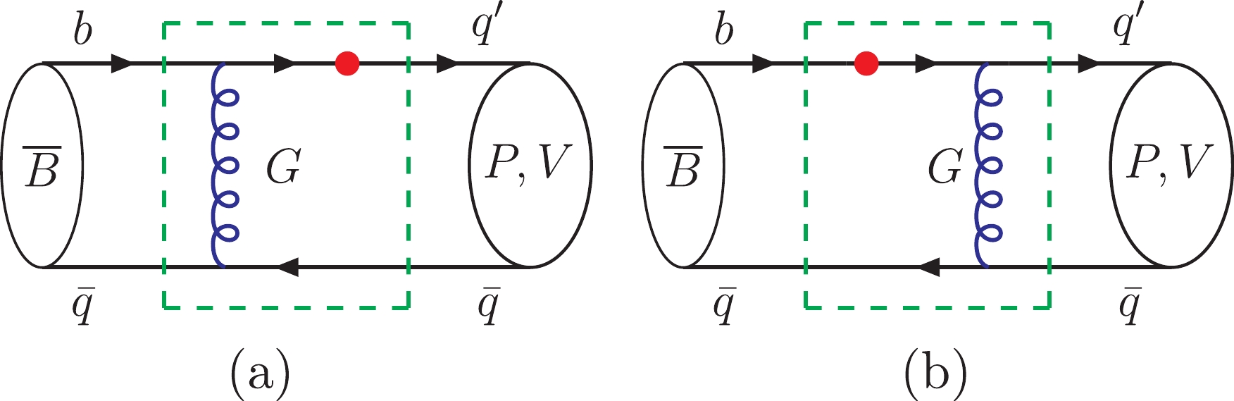
Figure 2.(color online) Diagrams contributing to the
$ \overline{B} {\to} P $ Vtransition with the PQCD approach, where the dots denote an appropriate diquark current interaction, and the dashed boxes represent the scattering amplitudes.It is well known that the two form factors,
$ F_{1}(q^{2}) $ and$ A_{0}(q^{2}) $ corresponding to the vector and axial-vector currents of the weak interactions, respectively, are directly related to$ B {\to} PV $ decays. The detailed definitions and explicit expressions of form factors can be found in Ref. [43], where the contributions from the higher twist DAs are considered properly. The dependences of form factors on certain input parameters are shown inFig. 3. It is clearly shown inFig. 3that (1) the form factors$ F_{1} $ and$ A_{0} $ are highly sensitive to the shape parameter$ {\omega}_{B} $ ofBmesonic WFs and the contributions from$ {\phi}_{B2} $ . In general, the values of the form factors$ F_{1} $ and$ A_{0} $ decrease with increasing$ {\omega}_{B} $ . This type of regular phenomenon has also been found in previous studies [40–42,44,45,48]. (2) In addition, the form factor$ F_{1} $ is also dependent on the value of the chiral parameter$ {\mu}_{P} $ . For a more comprehensive analysis, the numerical results of the form factors with specific inputs are listed inTable 2. It is clear fromTable 2that (1) when the contributions from$ {\phi}_{B2} $ are not considered, the total share of the form factor$ F_{1} $ from the twist-3 DAs$ {\phi}_{P}^{p,t} $ of the recoiled light pseudoscalar meson far outweighs those from the leading twist DAs$ {\phi}_{P}^{a} $ and account for more than$ 60 $ %. The total share of the form factor$ A_{0} $ from the twist-3 DAs$ {\phi}_{V}^{t,s} $ of the recoiled vector meson, which is approximately$ 60 $ %, far exceeds those from the twist-2 DAs$ {\phi}_{V}^{v} $ . (2) When only the contributions from the twist-2 DAs$ {\phi}_{P}^{a} $ and$ {\phi}_{V}^{v} $ are considered, the share of the form factors$ F_{1} $ and$ A_{0} $ from theBmesonic WFs$ {\phi}_{B2} $ is approximately$ 40 $ %. (3) When the contributions from both the twist-2 and twist-3 DAs$ {\phi}_{P}^{a,p,t} $ and$ {\phi}_{V}^{v,t,s} $ are considered, the share of the form factors$ F_{1} $ and$ A_{0} $ from theBmesonic WFs$ {\phi}_{B2} $ is approximately$ 20 $ %. The contributions from$ {\phi}_{B2} $ to the form factors have been investigated in previous studies [40–46]. The general consensus seems to be that the unnegligible contributions from$ {\phi}_{B2} $ to the form factors should be given due attention. Here, we would like to note that for arguments on the reliability of the perturbative calculation of the form factors using the PQCD approach, which is not the focus of this study, one can refer to detailed analyses, for example, in Refs. [43–45].$ F_{1}^{B{\to}{\pi}}(0) $ 

$ {\phi}_{\pi}^{a} $ 

$ {\phi}_{\pi}^{p} $ 

$ {\phi}_{\pi}^{t} $ 

$ {\Sigma}_{\pi} $ 

$ {\phi}_{\pi}^{a}/{\Sigma}_{\pi} $ 

$ {\phi}_{\pi}^{p}/{\Sigma}_{\pi} $ 

$ {\phi}_{\pi}^{t}/{\Sigma}_{\pi} $ 

$ {\phi}_{B1} $ 

$ 0.064 $ 

$ 0.106 $ 

$ 0.019 $ 

$ 0.188 $ 

$ 34.0 $ 

$ 56.0 $ 

$ 9.9 $ 

$ {\phi}_{B2} $ 

$ 0.045 $ 

$ -0.003 $ 

$ -0.000 $ 

$ 0.042 $ 

$ 107.5 $ 

$ -6.8 $ 

$ -0.7 $ 

$ {\Sigma}_{B} $ 

$ 0.109 $ 

$ 0.103 $ 

$ 0.018 $ 

$ 0.230 $ 

$ 47.4 $ 

$ 44.7 $ 

$ 8.0 $ 

$ {\phi}_{B2}/{\Sigma}_{B} $ 

$ 41.1 $ 

$ -2.8 $ 

$ -1.6 $ 

$ 18.1 $ 

$ F_{1}^{B{\to}K}(0) $ 

$ {\phi}_{K}^{a} $ 

$ {\phi}_{K}^{p} $ 

$ {\phi}_{K}^{t} $ 

$ {\Sigma}_{K} $ 

$ {\phi}_{K}^{a}/{\Sigma}_{K} $ 

$ {\phi}_{K}^{p}/{\Sigma}_{K} $ 

$ {\phi}_{K}^{t}/{\Sigma}_{K} $ 

$ {\phi}_{B1} $ 

$ 0.081 $ 

$ 0.131 $ 

$ 0.018 $ 

$ 0.230 $ 

$ 35.3 $ 

$ 56.9 $ 

$ 7.8 $ 

$ {\phi}_{B2} $ 

$ 0.056 $ 

$ -0.004 $ 

$ -0.000 $ 

$ 0.053 $ 

$ 107.3 $ 

$ -6.9 $ 

$ -0.5 $ 

$ {\Sigma}_{B} $ 

$ 0.138 $ 

$ 0.127 $ 

$ 0.018 $ 

$ 0.282 $ 

$ 48.7 $ 

$ 45.0 $ 

$ 6.3 $ 

$ {\phi}_{B2}/{\Sigma}_{B} $ 

$ 41.0 $ 

$ -2.8 $ 

$ -1.4 $ 

$ 18.6 $ 

$ A_{0}^{B{\to}{\rho}}(0) $ 

$ {\phi}_{\rho}^{v} $ 

$ {\phi}_{\rho}^{t} $ 

$ {\phi}_{\rho}^{s} $ 

$ {\Sigma}_{\rho} $ 

$ {\phi}_{\rho}^{v}/{\Sigma}_{\rho} $ 

$ {\phi}_{\rho}^{t}/{\Sigma}_{\rho} $ 

$ {\phi}_{\rho}^{s}/{\Sigma}_{\rho} $ 

$ {\phi}_{B1} $ 

$ 0.097 $ 

$ 0.090 $ 

$ 0.044 $ 

$ 0.231 $ 

$ 41.8 $ 

$ 39.1 $ 

$ 19.1 $ 

$ {\phi}_{B2} $ 

$ 0.069 $ 

$ -0.002 $ 

$ -0.001 $ 

$ 0.067 $ 

$ 103.6 $ 

$ -2.7 $ 

$ -0.9 $ 

$ {\Sigma}_{B} $ 

$ 0.166 $ 

$ 0.088 $ 

$ 0.044 $ 

$ 0.298 $ 

$ 55.7 $ 

$ 29.7 $ 

$ 14.6 $ 

$ {\phi}_{B2}/{\Sigma}_{B} $ 

$ 41.8 $ 

$ -2.0 $ 

$ -1.4 $ 

$ 22.4 $ 

$ A_{0}^{B{\to}K^{\ast}}(0) $ 

$ {\phi}_{K^{\ast}}^{v} $ 

$ {\phi}_{K^{\ast}}^{t} $ 

$ {\phi}_{K^{\ast}}^{s} $ 

$ {\Sigma}_{K^{\ast}} $ 

$ {\phi}_{K^{\ast}}^{v}/{\Sigma}_{K^{\ast}} $ 

$ {\phi}_{K^{\ast}}^{t}/{\Sigma}_{K^{\ast}} $ 

$ {\phi}_{K^{\ast}}^{s}/{\Sigma}_{K^{\ast}} $ 

$ {\phi}_{B1} $ 

$ 0.098 $ 

$ 0.106 $ 

$ 0.052 $ 

$ 0.256 $ 

$ 38.1 $ 

$ 41.4 $ 

$ 20.5 $ 

$ {\phi}_{B2} $ 

$ 0.070 $ 

$ -0.003 $ 

$ -0.001 $ 

$ 0.067 $ 

$ 104.5 $ 

$ -3.7 $ 

$ -0.8 $ 

$ {\Sigma}_{B} $ 

$ 0.168 $ 

$ 0.104 $ 

$ 0.052 $ 

$ 0.323 $ 

$ 52.0 $ 

$ 32.0 $ 

$ 16.0 $ 

$ {\phi}_{B2}/{\Sigma}_{B} $ 

$ 42.0 $ 

$ -2.4 $ 

$ -1.1 $ 

$ 20.9 $ 

Table 2.Contributions from different twist hadronic DAs to the form factors
$ F_{1}(q^{2}) $ and$ A_{0}(q^{2}) $ at$ q^{2} = 0 $ using the PQCD approach, where$ {\omega}_{B} = 0.4 $ GeV,$ {\mu}_{P} = 1.4 $ GeV,$ {\Sigma}_{P} = {\phi}_{P}^{a} + {\phi}_{P}^{p} + {\phi}_{P}^{t} $ ,$ {\Sigma}_{V} = {\phi}_{V}^{v} + {\phi}_{V}^{t} + {\phi}_{V}^{s} $ , and$ {\Sigma}_{B} = {\phi}_{B1} + {\phi}_{B2} $ . The ratio$ {\phi}_{i}/{\Sigma}_{j} $ is expressed as a percentage.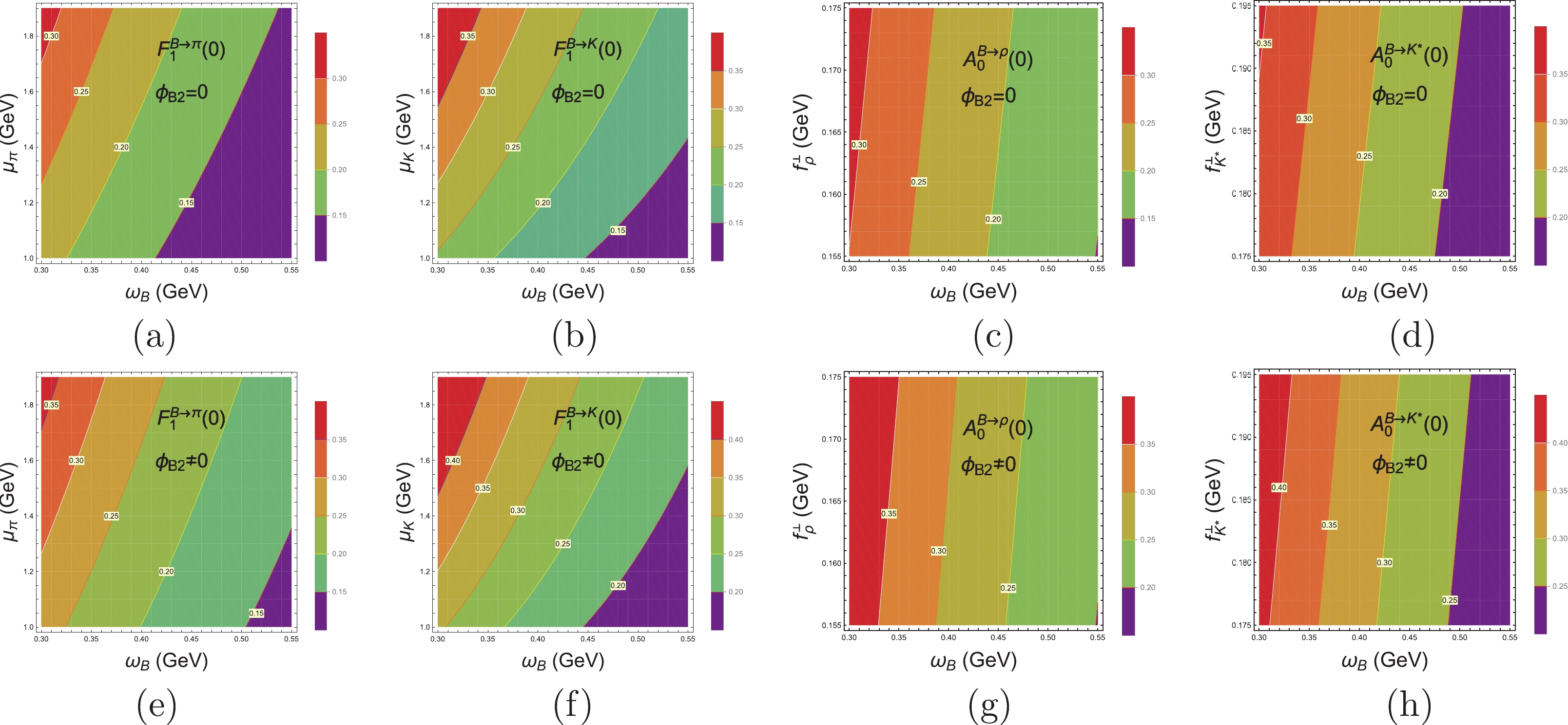
Figure 3.(color online) Contour plot of the form factors
$ F_{1}(q^{2}) $ and$ A_{0}(q^{2}) $ at$ q^{2} = 0 $ , where the values in (a, b, c, d) and (e, f, g, h) are calculated without and with contributions from$ {\phi}_{B2} $ . -
According to the above analysis, it is clear that the contributions from higher twist DAs are important to HMEs for nonleptonicBdecays using the PQCD approach. In most phenomenological studies of
$ B {\to} PV $ decays with the PQCD approach, the shares of both the twist-2 DAs ($ {\phi}_{P}^{a} $ and$ {\phi}_{V}^{v} $ ) and twist-3 DAs ($ {\phi}_{P}^{p,t} $ and$ {\phi}_{V}^{t,s} $ ) for the final mesons have been carefully and commonly considered, such as in Refs. [48–55]. In contrast, the possible influence of theBmesonic WFs$ {\phi}_{B}^{-} $ or$ {\phi}_{B2} $ on nonleptonicBdecays garners significantly less attention. In this paper, our main purpose is to investigate the effects of theBmesonic WFs$ {\phi}_{B2} $ on$ B {\to} PV $ decays using the PQCD approach.Leading order Feynman diagrams are shown inFig. 4. The analytical expressions of each subdiagram amplitude are listed in Appendix B. It is clearly seen that (1) for the factorizable annihilation diagrams (e) and (f), the initialBmeson is completely disconnected from the final state
$ PV $ system, where the disconnectedBmeson corresponds to its decay constant and should have nothing to do with its WFs$ {\phi}_{B2} $ . These arguments are fully verified by Eqs. (B31)–(B42). (2) For the emission diagrams (a-d) and the nonfactorizable annihilation diagrams (g-h), theBmeson always connects with either one or two of the final states via one-gluon-exchange interactions. Therefore, these corresponding amplitudes would generally be affected by theBmesonic WFs$ {\phi}_{B2} $ and should be updated accordingly.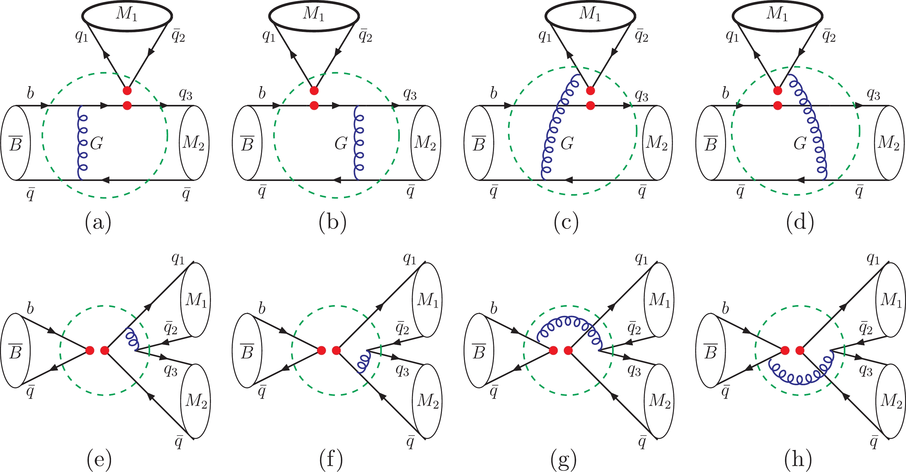
Figure 4.(color online) Feynman diagrams contributing to
$ \overline{B} {\to} PV $ decays with the PQCD approach, where$ M_{1,2} = P $ andV, the dots denote appropriate interactions, and the dashed circles represent the scattering amplitudes. (a) and (b) are factorizable emission diagrams. (c) and (d) are nonfactorizable emission diagrams. (e) and (f) are factorizable annihilation diagrams. (g) and (h) are nonfactorizable annihilation diagrams.The decay amplitudes for
$ B {\to} PV $ decays with the PQCD approach are expressed as the sum of a series of multidimensional convolutions,$ \begin{aligned}[b] & {\cal A}(B{\to}PV)\, =\, {\langle}PV{\vert}{\cal H}_{\rm eff}{\vert}B{\rangle} \\ =& \frac{G_{\rm F}}{\sqrt{2}}\,\sum\limits_{i}\,{\cal F}_{i} {\int}\,{\rm d}x_{1}\,{\rm d}x_{2}\,{\rm d}x_{3}\,{\rm d}b_{1}\,{\rm d}b_{2}\,{\rm d}b_{3}\,\\&\times {\cal T}_{i}(t_{i},x_{1},b_{1},x_{2},b_{2},x_{3},b_{3}) \\ & \times C_{i}(t_{i})\, {\Phi}_{B}(x_{1},b_{1}){\rm e}^{-S_{B}} \\&\times \, {\Phi}_{P}(x_{2},b_{2})\,{\rm e}^{-S_{P}}\, {\Phi}_{V}(x_{3},b_{3})\,{\rm e}^{-S_{V}} , \end{aligned} $

(39) where
$ {\cal F}_{i} $ is the CKM factor, and the rescattering functions$ {\cal T}_{i} $ are represented by the dashed circles inFig. 4. The calculation expressions for the$ B {\to} PV $ decays are listed in detail in Appendix A.In the rest frame of theBmeson, the
$C P$ -averaged branching ratios are defined as$ {\cal B}\, =\, \frac{{\tau}_{B}}{16{\pi}}\, \frac{p_{\rm cm}}{m_{B}^{2}}\, \big\{ {\vert}{\cal A}(B{\to}f){\vert}^{2}+ {\vert}{\cal A}(\overline{B}{\to}\bar{f}){\vert}^{2} \big\} , $

(40) where
$ {\tau}_{B} $ is the lifetime of theBmeson,$ {\tau}_{B_{u}} = 1.638(4) $ ps, and$ {\tau}_{B_{d}} = 1.519(4) $ ps [5].$ p_{\rm cm} $ is the common center-of-mass momentum of final states.For charged
$ B_{u} $ meson decays, direct$C P$ violating asymmetry arising from interferences among different amplitudes is defined as$\begin{aligned}[b] {\cal A}_{CP}\, =& \frac{{\Gamma}(B^-{\to}f)-{\Gamma}(B^+{\to}\bar{f})} {{\Gamma}(B^-{\to}f)+{\Gamma}(B^+{\to}\bar{f})} \\ =\,& \frac{{\vert}\mathcal{A}(B^-{\to}f){\vert}^{2} -{\vert}\mathcal{A}(B^+{\to}\bar{f}){\vert}^{2}} {{\vert}\mathcal{A}(B^-{\to}f){\vert}^{2} +{\vert}\mathcal{A}(B^+{\to}\bar{f}){\vert}^{2}} . \end{aligned} $

(41) For neutral
$ B_{d} $ meson decays, the effects of$ B^{0} $ -$ \overline{B}^{0} $ mixing should be considered. Time-dependent$C P$ violating asymmetry is defined as$ {\cal A}_{CP}(t)\, =\, \frac{ {\Gamma}(\overline{B}^{0}(t){\to}f) - {\Gamma}(B^{0}(t){\to}\bar{f})} { {\Gamma}(\overline{B}^{0}(t){\to}f) + {\Gamma}(B^{0}(t){\to}\bar{f})} . $

(42) $C P$ violating asymmetries can, in principle, be divided into three cases according to the final states [5,63,64]. For the sake of simplification, the following conventional symbols will be defined and used:$ A_{f}\, =\, {\cal A}(B^{0}(0){\to}f), \qquad \bar{A}_{f}\, =\, {\cal A}(\overline{B}^{0}(0){\to}f) , $

(43) $ A_{\bar{f}}\, =\, {\cal A}(B^{0}(0){\to}\bar{f}), \qquad \bar{A}_{\bar{f}}\, =\, {\cal A}(\overline{B}^{0}(0){\to}\bar{f}) . $

(44) ● Case 1: The final states originate from either
$ B^{0} $ decays or$ \overline{B}^{0} $ decays, but not both, that is,$ \overline{B}^{0} {\to} f $ and$ B^{0} {\to} \bar{f} $ with$ f {\ne} \bar{f} $ , for example, the$ \overline{B}^{0} {\to} {\pi}^{+}K^{{\ast}-} $ decay. The$ C P $ asymmetries are immune to$ B^{0} $ -$ \overline{B}^{0} $ mixing and have a similar definition to the direct$ C P $ asymmetry in Eq. (41).● Case 2: The final states are the eigenstates of the
$C P$ transformation, that is,$ f^{CP} = {\eta}_{f}\,\bar{f} $ with the eigenvalue$ {\vert}{\eta}_{f}{\vert} = 1 $ . The final states can originate from both$ B^{0} $ decays and$ \overline{B}^{0} $ decays, that is,$ \overline{B}^{0} {\to} f {\gets} B^{0} $ , for example, the$ \overline{B}^{0} {\to} {\pi}^{0}{\rho}^{0} $ decay.For
$ B^{0} $ -$ \overline{B}^{0} $ mixing, the SM predicts that the ratio of the decay width difference$ {\Delta}{\Gamma} $ of mass eigenstates to the total decay width$ {\Gamma} $ is small, that is,$ {\Delta}{\Gamma}/{\Gamma} = 0.001{\pm}0.010 $ , from data [5]. In the most general calculation, it is usually assumed that$ {\Delta}{\Gamma} = 0 $ ; thus, the$C P$ asymmetries can be expressed as [5]$ {\cal A}_{CP}(t)\, =\, S_{f}\,{\sin}({\Delta}m\,t) -C_{f}\,{\cos}({\Delta}m\,t) , $

(45) $ S_{f}\, =\, \frac{ 2\,{\cal I}m({\lambda}_{f}) } { 1+{\vert}{\lambda}_{f}{\vert}^{2} }, \quad C_{f}\, =\, \frac{ 1-{\vert}{\lambda}_{f}{\vert}^{2} } { 1+{\vert}{\lambda}_{f}{\vert}^{2} }, \quad {\lambda}_{f}\, =\, \frac{ q }{ p }\, \frac{ \bar{A}_{f} }{ A_{f} } , $

(46) where
$ q/p = V_{tb}^{\ast}\,V_{td}/V_{tb}\,V_{td}^{\ast} $ describes$ B^{0} $ -$ \overline{B}^{0} $ mixing. Sometimes, time-integrated$C P$ asymmetries are written as$ {\cal A}_{CP} = \frac{ {\int}_{0}^{\infty}{\rm d}t\,{\Gamma}(\overline{B}^{0}(t){\to}f) - {\int}_{0}^{\infty}{\rm d}t\,{\Gamma}(B^{0}(t){\to}\bar{f}) } { {\int}_{0}^{\infty}{\rm d}t\,{\Gamma}(\overline{B}^{0}(t){\to}f) + {\int}_{0}^{\infty}{\rm d}t\,{\Gamma}(B^{0}(t){\to}\bar{f}) } $

(47) $ \begin{array}{*{20}{l}}\qquad = \dfrac{ x }{ 1+x^{2} }\,S_{f} -\dfrac{ 1 }{ 1+x^{2} }\,C_{f} , \end{array} $

(48) with
$ x = {\Delta}m/{\Gamma} = 0.769(4) $ [5] for the$ B^{0} $ -$ \overline{B}^{0} $ system, where$ {\Delta}m = 0.5065(19)\,{\rm ps}^{-1} $ [5] is the mass difference of the mass eigenstates.● Case 3: The final states are not the eigenstates of the
$C P$ transformation; however, bothfand$ \bar{f} $ are the common final states of$ \overline{B}^{0} $ and$ B^{0} $ , that is,$ \overline{B}^{0} {\to} $ (f&$ \bar{f} $ )$ {\gets} B^{0} $ , for example, the$ \overline{B}^{0} {\to} {\pi}^{+}{\rho}^{-} $ and$ {\pi}^{-}{\rho}^{+} $ decays.The four time-dependent partial decay widths can be expressed as [63,64]
$ \begin{aligned}[b]{\Gamma}(B^{0}(t){\to}f)\, =&\, \frac{1}{2}\, {\rm e}^{-{\Gamma}\,t}\, \big( {\vert}A_{f}{\vert}^{2} +{\vert}\bar{A}_{f}{\vert}^{2} \big)\, \\&\times\Big\{ 1 +a_{{\epsilon}^{\prime}}\,{\cos}({\Delta}m\,t) +a_{{\epsilon}+{\epsilon}^{\prime}}\, {\sin}({\Delta}m\,t) \Big\} ,\end{aligned} $

(49) $ \begin{aligned}[b] {\Gamma}(B^{0}(t){\to}\bar{f})\, =&\, \frac{1}{2}\, {\rm e}^{-{\Gamma}\,t}\, \big( {\vert}\bar{A}_{\bar{f}}{\vert}^{2} +{\vert}A_{\bar{f}}{\vert}^{2} \big)\,\\&\times \Big\{ 1 +\bar{a}_{{\epsilon}^{\prime}}\,{\cos}({\Delta}m\,t) +\bar{a}_{{\epsilon}+{\epsilon}^{\prime}}\, {\sin}({\Delta}m\,t) \Big\} ,\end{aligned} $

(50) $ \begin{aligned}[b] {\Gamma}(\overline{B}^{0}(t){\to}f)\, =&\, \frac{1}{2}\, {\rm e}^{-{\Gamma}\,t}\, \big( {\vert}A_{f}{\vert}^{2} +{\vert}\bar{A}_{f}{\vert}^{2} \big)\, \\&\times\Big\{ 1 -a_{{\epsilon}^{\prime}}\,{\cos}({\Delta}m\,t) -a_{{\epsilon}+{\epsilon}^{\prime}}\, {\sin}({\Delta}m\,t) \Big\} , \end{aligned}$

(51) $ \begin{aligned}[b] {\Gamma}(\overline{B}^{0}(t){\to}\bar{f}) \, =&\, \frac{1}{2}\, {\rm e}^{-{\Gamma}\,t}\, \big( {\vert}\bar{A}_{\bar{f}}{\vert}^{2} +{\vert}A_{\bar{f}}{\vert}^{2} \big)\,\\&\times \Big\{ 1 -\bar{a}_{{\epsilon}^{\prime}}\,{\cos}({\Delta}m\,t) -\bar{a}_{{\epsilon}+{\epsilon}^{\prime}}\, {\sin}({\Delta}m\,t) \Big\} , \end{aligned} $

(52) with the following definitions:
$ a_{{\epsilon}^{\prime}}\, =\, \frac{ 1-{\vert}{\lambda}_{f}{\vert}^{2} } { 1+{\vert}{\lambda}_{f}{\vert}^{2} }, \quad a_{{\epsilon}+{\epsilon}^{\prime}}\, =\, \frac{ -2\,{\cal I}m({\lambda}_{f}) } { 1+{\vert}{\lambda}_{f}{\vert}^{2} }, \quad {\lambda}_{f}\, =\, \frac{ V_{tb}^{\ast}\,V_{td} }{ V_{tb}\,V_{td}^{\ast} }\, \frac{ \bar{A}_{f} }{ A_{f} } , $

(53) $ \bar{a}_{{\epsilon}^{\prime}}\, =\, \frac{ 1-{\vert}\bar{\lambda}_{f}{\vert}^{2} } { 1+{\vert}\bar{\lambda}_{f}{\vert}^{2} }, \quad \bar{a}_{{\epsilon}+{\epsilon}^{\prime}}\, =\, \frac{ -2\,{\cal I}m(\bar{\lambda}_{f}) } { 1+{\vert}\bar{\lambda}_{f}{\vert}^{2} }, \quad \bar{\lambda}_{f}\, =\, \frac{ V_{tb}^{\ast}\,V_{td} }{ V_{tb}\,V_{td}^{\ast} }\, \frac{ \bar{A}_{\bar{f}} }{ A_{\bar{f}} } . $

(54) Besides
$ {\cal A}_{CP} $ in Eq.(48),$C P$ asymmetries can also be expressed by the physical quantities$ a_{{\epsilon}^{\prime}} $ ,$ a_{{\epsilon}+{\epsilon}^{\prime}} $ ,$ \bar{a}_{{\epsilon}^{\prime}} $ , and$ \bar{a}_{{\epsilon}+{\epsilon}^{\prime}} $ .According to the previous analysis of the form factors inFig. 3, it is natural to suppose that the theoretical results of the branching ratios would be strongly dependent on the shape parameter
$ {\omega}_{B} $ . In this paper, we optimize the parameter$ {\omega}_{B} $ using the minimum$ {\chi}^{2} $ method:$ {\chi}^{2}\, =\, \sum\limits_{i}{\chi}^{2}_{i}\, =\, \sum\limits_{i} \frac{ ({\cal B}_{i}^{\rm th.}-{\cal B}_{i}^{\rm exp.})^{2} } { {\sigma}_{i}^{2} } , $

(55) where
$ {\cal B}_{i}^{\rm th.} $ and$ {\cal B}_{i}^{\rm exp.} $ denote the theoretical results and experimental data on the branching ratio, respectively.$ {\sigma}_{i} $ denotes the errors on the experimental measurements. The distribution of$ {\chi}^{2} $ vs the shape parameter$ {\omega}_{B} $ is shown inFig. 5, where the contributions from theBmesonic WFs$ {\phi}_{B2} $ are considered. Three optimal scenarios of the shape parameter$ {\omega}_{B} $ corresponding to experimental data from the PDG, BaBar, and Belle groups are obtained with the chiral mass$ {\mu}_{P} = 1.4 $ GeV, that is,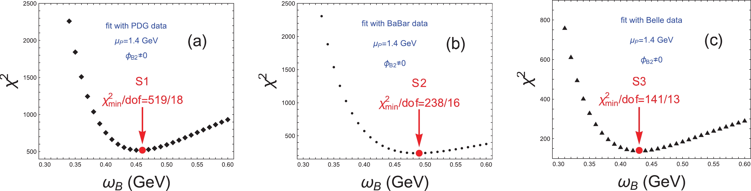
Figure 5.(color online) Distribution of
$ {\chi}^{2} $ vs the shape parameter$ {\omega}_{B} $ , where the red points at the arrowheads correspond to the optimal values.● Scenario 1 (S1):
$ {\omega}_{B} = 0.46 $ GeV from PDG data with$ {\chi}^{2}_{\rm min.} $ /dof$ {\approx} 519/18 {\approx} 29 $ ,● Scenario 2 (S2):
$ {\omega}_{B} = 0.49 $ GeV from BaBar data with$ {\chi}^{2}_{\rm min.} $ /dof$ {\approx} 238/16 {\approx} 15 $ ,● Scenario 3 (S3):
$ {\omega}_{B} = 0.43 $ GeV from Belle data with$ {\chi}^{2}_{\rm min.} $ /dof$ {\approx} 141/13 {\approx} 11 $ .As is well known, the errors of the PDG group from a weighted average of selected data are generally smaller than those of any independent experimental groups. Therefore, it is clear from Eq. (55) that the relatively smaller (larger) errors on the PDG (Belle) data result in the relatively larger (smaller) value of
$ {\chi}^{2}_{\rm min.} $ /dof.The numerical results of the
$C P$ -averaged branching ratios for three scenarios (S1, S2, and S3) using the PQCD approach with experimental data are presented inTables 3and4, and the previous PQCD results without contributions from theBmesonic WFs$ {\phi}_{B2} $ are listed inTable 5. To obtain a clear and comprehensive impression of the agreement between the theoretical and experimental results, the$ {\chi}_{i}^{2} $ distributions are illustrated inFig. 6. The results of the$C P$ asymmetries are presented inTables 6,7, and8. It should be noted that the uncertainties on our results only originate from the parameters$ {\omega}_{B} $ and$ {\mu}_{P} $ based on the previous analysis of form factors. Uncertainties from other factors, such as the Gegenbauer moments①and different models of the mesonic WFs, are not carefully scrutinized here, but deserve a more dedicated study.mode $ B^{-} {\to} {\pi}^{-}{\rho}^{0} $ 

$ B^{-} {\to} {\pi}^{0}{\rho}^{-} $ 

$ B^{-} {\to} {\pi}^{-}{\omega} $ 

$ B^{-} {\to} {\pi}^{-}{\phi} $ 

data PDG $ 8.3{\pm}1.2 $ 

$ 10.9{\pm}1.4 $ 

$ 6.9{\pm}0.5 $ 

$ (3.2{\pm}1.5){\times}10^{-2} $ 

S1 $ {\phi}_{B1} $ +

$ {\phi}_{B2} $ 

$ 4.25^{+ 0.22 + 0.01 }_{- 0.21 - 0.00 } $ 

$ 6.91^{+ 0.39 + 0.46 }_{- 0.37 - 0.45 } $ 

$ 3.83^{+ 0.20 + 0.01 }_{- 0.19 - 0.01 } $ 

$ 4.9^{+ 0.4 + 0.6 }_{- 0.4 - 0.5 }{\times}10^{-2} $ 

$ {\phi}_{B1} $ 

$ 2.66^{+ 0.15 + 0.01 }_{- 0.14 - 0.01 } $ 

$ 4.56^{+ 0.28 + 0.38 }_{- 0.26 - 0.36 } $ 

$ 2.47^{+ 0.14 + 0.01 }_{- 0.13 - 0.01 } $ 

$ 4.2^{+ 0.3 + 0.5 }_{- 0.3 - 0.5 }{\times}10^{-2} $ 

data BaBar $ 8.1{\pm}1.7 $ 

$ 10.2{\pm}1.7 $ 

$ 6.7{\pm}0.6 $ 

S2 $ {\phi}_{B1} $ +

$ {\phi}_{B2} $ 

$ 3.66^{+ 0.19 + 0.01 }_{- 0.18 - 0.00 } $ 

$ 5.87^{+ 0.32 + 0.38 }_{- 0.30 - 0.37 } $ 

$ 3.28^{+ 0.17 + 0.01 }_{- 0.16 - 0.01 } $ 

$ 3.9^{+ 0.3 + 0.4 }_{- 0.3 - 0.4 }{\times}10^{-2} $ 

$ {\phi}_{B1} $ 

$ 2.26^{+ 0.12 + 0.01 }_{- 0.12 - 0.01 } $ 

$ 3.83^{+ 0.22 + 0.31 }_{- 0.21 - 0.30 } $ 

$ 2.10^{+ 0.12 + 0.00 }_{- 0.11 - 0.00 } $ 

$ 3.3^{+ 0.3 + 0.4 }_{- 0.3 - 0.4 }{\times}10^{-2} $ 

data Belle $ 8.0{\pm}2.4 $ 

$ 13.2{\pm}3.0 $ 

$ 6.9{\pm}0.8 $ 

S3 $ {\phi}_{B1} $ +

$ {\phi}_{B2} $ 

$ 4.96^{+ 0.26 + 0.01 }_{- 0.25 - 0.00 } $ 

$ 8.17^{+ 0.48 + 0.56 }_{- 0.45 - 0.54 } $ 

$ 4.47^{+ 0.24 + 0.01 }_{- 0.23 - 0.01 } $ 

$ 6.2^{+ 0.5 + 0.7 }_{- 0.5 - 0.7 }{\times}10^{-2} $ 

$ {\phi}_{B1} $ 

$ 3.13^{+ 0.18 + 0.01 }_{- 0.17 - 0.01 } $ 

$ 5.45^{+ 0.34 + 0.46 }_{- 0.32 - 0.44 } $ 

$ 2.91^{+ 0.17 + 0.01 }_{- 0.16 - 0.01 } $ 

$ 5.3^{+ 0.4 + 0.6 }_{- 0.4 - 0.6 }{\times}10^{-2} $ 

mode $ B^{-} {\to} K^{-}K^{{\ast}0} $ 

$ B^{-} {\to} K^{0}K^{{\ast}-} $ 

$ B^{-} {\to} {\pi}^{0}K^{{\ast}-} $ 

$ B^{-} {\to} K^{-}{\rho}^{0} $ 

data PDG $ 0.59{\pm}0.08 $ 

$ 6.8{\pm}0.9 $ 

$ 3.7{\pm}0.5 $ 

S1 $ {\phi}_{B1} $ +

$ {\phi}_{B2} $ 

$ 0.35^{+ 0.02 + 0.05 }_{- 0.02 - 0.05 } $ 

$ 4.7^{+ 0.1 + 1.3 }_{- 0.1 - 0.8 }{\times}10^{-2} $ 

$ 2.90^{+ 0.19 + 0.22 }_{- 0.18 - 0.22 } $ 

$ 1.04^{+ 0.01 + 0.03 }_{- 0.01 - 0.00 } $ 

$ {\phi}_{B1} $ 

$ 0.24^{+ 0.02 + 0.04 }_{- 0.01 - 0.04 } $ 

$ 4.8^{+ 0.1 + 1.3 }_{- 0.1 - 1.0 }{\times}10^{-2} $ 

$ 1.96^{+ 0.14 + 0.19 }_{- 0.13 - 0.18 } $ 

$ 0.88^{+ 0.01 + 0.03 }_{- 0.01 - 0.01 } $ 

data BaBar $ 6.4{\pm}1.0 $ 

$ 3.56{\pm}0.73 $ 

S2 $ {\phi}_{B1} $ +

$ {\phi}_{B2} $ 

$ 0.29^{+ 0.02 + 0.04 }_{- 0.02 - 0.04 } $ 

$ 4.4^{+ 0.1 + 1.0 }_{- 0.1 - 0.7 }{\times}10^{-2} $ 

$ 2.40^{+ 0.15 + 0.18 }_{- 0.14 - 0.18 } $ 

$ 1.01^{+ 0.01 + 0.02 }_{- 0.01 - 0.00 } $ 

$ {\phi}_{B1} $ 

$ 0.19^{+ 0.01 + 0.03 }_{- 0.01 - 0.03 } $ 

$ 4.5^{+ 0.1 + 1.1 }_{- 0.1 - 0.8 }{\times}10^{-2} $ 

$ 1.61^{+ 0.11 + 0.15 }_{- 0.10 - 0.15 } $ 

$ 0.86^{+ 0.01 + 0.02 }_{- 0.01 - 0.01 } $ 

data Belle $ 3.89{\pm}0.64 $ 

S3 $ {\phi}_{B1} $ +

$ {\phi}_{B2} $ 

$ 0.42^{+ 0.03 + 0.06 }_{- 0.03 - 0.06 } $ 

$ 5.1^{+ 0.2 + 1.6 }_{- 0.1 - 1.0 }{\times}10^{-2} $ 

$ 3.52^{+ 0.24 + 0.27 }_{- 0.22 - 0.26 } $ 

$ 1.08^{+ 0.02 + 0.03 }_{- 0.01 - 0.00 } $ 

$ {\phi}_{B1} $ 

$ 0.29^{+ 0.02 + 0.05 }_{- 0.02 - 0.05 } $ 

$ 5.3^{+ 0.2 + 1.6 }_{- 0.2 - 1.2 }{\times}10^{-2} $ 

$ 2.41^{+ 0.18 + 0.23 }_{- 0.16 - 0.22 } $ 

$ 0.91^{+ 0.01 + 0.03 }_{- 0.01 - 0.01 } $ 

mode $ B^{-} {\to} K^{-}{\omega} $ 

$ B^{-} {\to} {\pi}^{-}\overline{K}^{{\ast}0} $ 

$ B^{-} {\to} \overline{K}^{0}{\rho}^{-} $ 

$ B^{-} {\to} K^{-}{\phi} $ 

data PDG $ 6.5{\pm}0.4 $ 

$ 10.1{\pm}0.8 $ 

$ 7.3{\pm}1.2 $ 

$ 8.8{\pm}0.7 $ 

S1 $ {\phi}_{B1} $ +

$ {\phi}_{B2} $ 

$ 3.43^{+ 0.17 + 0.26 }_{- 0.16 - 0.30 } $ 

$ 4.44^{+ 0.31 + 0.44 }_{- 0.28 - 0.42 } $ 

$ 1.36^{+ 0.00 + 0.12 }_{- 0.00 - 0.05 } $ 

$ 13.48^{+ 0.96 + 2.32 }_{- 0.89 - 2.27 } $ 

$ {\phi}_{B1} $ 

$ 2.76^{+ 0.13 + 0.28 }_{- 0.12 - 0.30 } $ 

$ 3.04^{+ 0.22 + 0.36 }_{- 0.20 - 0.34 } $ 

$ 1.36^{+ 0.01 + 0.15 }_{- 0.01 - 0.09 } $ 

$ 9.50^{+ 0.73 + 1.94 }_{- 0.67 - 1.87 } $ 

data BaBar $ 6.3{\pm}0.6 $ 

$ 10.1{\pm}2.0 $ 

$ 6.5{\pm}2.2 $ 

$ 9.2{\pm}0.8 $ 

S2 $ {\phi}_{B1} $ +

$ {\phi}_{B2} $ 

$ 2.99^{+ 0.14 + 0.22 }_{- 0.13 - 0.25 } $ 

$ 3.65^{+ 0.24 + 0.36 }_{- 0.23 - 0.34 } $ 

$ 1.36^{+ 0.00 + 0.10 }_{- 0.00 - 0.04 } $ 

$ 11.00^{+ 0.77 + 1.87 }_{- 0.71 - 1.83 } $ 

$ {\phi}_{B1} $ 

$ 2.41^{+ 0.11 + 0.23 }_{- 0.10 - 0.25 } $ 

$ 2.48^{+ 0.17 + 0.29 }_{- 0.16 - 0.28 } $ 

$ 1.34^{+ 0.00 + 0.12 }_{- 0.00 - 0.07 } $ 

$ 7.64^{+ 0.57 + 1.55 }_{- 0.53 - 1.49 } $ 

data Belle $ 6.8{\pm}0.6 $ 

$ 9.67{\pm}1.10 $ 

$ 9.60{\pm}1.40 $ 

S3 $ {\phi}_{B1} $ +

$ {\phi}_{B2} $ 

$ 3.98^{+ 0.21 + 0.32 }_{- 0.19 - 0.36 } $ 

$ 5.44^{+ 0.39 + 0.53 }_{- 0.36 - 0.51 } $ 

$ 1.38^{+ 0.01 + 0.16 }_{- 0.01 - 0.07 } $ 

$ 16.60^{+ 1.21 + 2.89 }_{- 1.12 - 2.83 } $ 

$ {\phi}_{B1} $ 

$ 3.19^{+ 0.16 + 0.33 }_{- 0.15 - 0.36 } $ 

$ 3.76^{+ 0.29 + 0.44 }_{- 0.26 - 0.42 } $ 

$ 1.38^{+ 0.01 + 0.18 }_{- 0.01 - 0.11 } $ 

$ 11.88^{+ 0.93 + 2.43 }_{- 0.86 - 2.35 } $ 

Table 3.
$C P$ -averaged branching ratios (in the unit of$ 10^{-6} $ ) for$ B_{u} {\to} PV $ decays. The central theoretical values are calculated with three scenario parameters of$ {\omega}_{B} $ to compare with data from the PDG, BaBar, and Belle groups [5]. The first theoretical uncertainties arise from variations in$ {\omega}_{B} = 0.46{\pm}0.01 $ GeV for S1,$ {\omega}_{B} = 0.49{\pm}0.01 $ GeV for S2, and$ {\omega}_{B} = 0.43{\pm}0.01 $ GeV for S3. The second theoretical uncertainties originate from variations in$ {\mu}_{P} = 1.4{\pm}0.1 $ GeV.mode $ \overline{B}^{0} {\to} {\pi}^{+}{\rho}^{-} $ 

$ \overline{B}^{0} {\to} {\pi}^{-}{\rho}^{+} $ 

$ \overline{B}^{0} {\to} {\pi}^{0}{\omega} $ 

$ \overline{B}^{0} {\to} {\pi}^{0}{\rho}^{0} $ 

$ \overline{B}^{0} {\to} {\pi}^{0}{\phi} $ 

data PDG $ 23.0{\pm}2.3 $ 

$<0.5 $ 

$ 2.0{\pm}0.5 $ 

$<0.15 $ 

S1 $ {\phi}_{B1} $ +

$ {\phi}_{B2} $ 

$ 10.11^{+ 0.59 + 0.60 }_{- 0.55 - 0.59 } $ 

$ 7.52^{+ 0.41 + 0.14 }_{- 0.38 - 0.13 } $ 

$ 0.16^{+ 0.01 + 0.00 }_{- 0.01 - 0.00 } $ 

$ 7.0^{+ 0.3 + 0.4 }_{- 0.3 - 0.3 }{\times}10^{-2} $ 

$ 2.3^{+ 0.2 + 0.3 }_{- 0.2 - 0.2 }{\times}10^{-2} $ 

$ {\phi}_{B1} $ 

$ 6.35^{+ 0.40 + 0.49 }_{- 0.37 - 0.47 } $ 

$ 4.58^{+ 0.26 + 0.12 }_{- 0.25 - 0.11 } $ 

$ 0.12^{+ 0.01 + 0.00 }_{- 0.01 - 0.00 } $ 

$ 5.8^{+ 0.3 + 0.2 }_{- 0.3 - 0.1 }{\times}10^{-2} $ 

$ 2.0^{+ 0.2 + 0.2 }_{- 0.2 - 0.2 }{\times}10^{-2} $ 

data BaBar $ 22.6{\pm}2.8 $ 

$<0.5 $ 

$ 1.4{\pm}0.7 $ 

$<0.28 $ 

S2 $ {\phi}_{B1} $ +

$ {\phi}_{B2} $ 

$ 8.56^{+ 0.48 + 0.50 }_{- 0.45 - 0.49 } $ 

$ 6.44^{+ 0.34 + 0.12 }_{- 0.32 - 0.11 } $ 

$ 0.13^{+ 0.01 + 0.00 }_{- 0.01 - 0.00 } $ 

$ 6.2^{+ 0.3 + 0.3 }_{- 0.2 - 0.3 }{\times}10^{-2} $ 

$ 1.8^{+ 0.1 + 0.2 }_{- 0.1 - 0.2 }{\times}10^{-2} $ 

$ {\phi}_{B1} $ 

$ 5.32^{+ 0.32 + 0.41 }_{- 0.30 - 0.39 } $ 

$ 3.88^{+ 0.22 + 0.10 }_{- 0.20 - 0.09 } $ 

$ 0.10^{+ 0.01 + 0.00 }_{- 0.01 - 0.00 } $ 

$ 5.1^{+ 0.2 + 0.1 }_{- 0.2 - 0.1 }{\times}10^{-2} $ 

$ 1.5^{+ 0.1 + 0.2 }_{- 0.1 - 0.2 }{\times}10^{-2} $ 

data Belle $ 22.6{\pm}4.5 $ 

$<2.0 $ 

$ 3.0{\pm}0.9 $ 

$<0.15 $ 

S3 $ {\phi}_{B1} $ +

$ {\phi}_{B2} $ 

$ 11.99^{+ 0.72 + 0.73 }_{- 0.67 - 0.71 } $ 

$ 8.82^{+ 0.49 + 0.17 }_{- 0.46 - 0.16 } $ 

$ 0.19^{+ 0.01 + 0.01 }_{- 0.01 - 0.01 } $ 

$ 8.0^{+ 0.4 + 0.4 }_{- 0.3 - 0.4 }{\times}10^{-2} $ 

$ 2.9^{+ 0.2 + 0.3 }_{- 0.2 - 0.3 }{\times}10^{-2} $ 

$ {\phi}_{B1} $ 

$ 7.64^{+ 0.49 + 0.60 }_{- 0.46 - 0.58 } $ 

$ 5.43^{+ 0.32 + 0.14 }_{- 0.30 - 0.14 } $ 

$ 0.14^{+ 0.01 + 0.01 }_{- 0.01 - 0.01 } $ 

$ 6.7^{+ 0.3 + 0.2 }_{- 0.3 - 0.2 }{\times}10^{-2} $ 

$ 2.5^{+ 0.2 + 0.3 }_{- 0.2 - 0.3 }{\times}10^{-2} $ 

mode $ \overline{B}^{0} {\to} \overline{K}^{0}K^{{\ast}0} $ 

$ \overline{B}^{0} {\to} K^{0}\overline{K}^{{\ast}0} $ 

$ \overline{B}^{0} {\to} {\pi}^{+}K^{{\ast}-} $ 

$ \overline{B}^{0} {\to} K^{-}{\rho}^{+} $ 

$ \overline{B}^{0} {\to} {\pi}^{0}\overline{K}^{{\ast}0} $ 

data PDG $<0.96 $ 

$ 7.5{\pm}0.4 $ 

$ 7.0{\pm}0.9 $ 

$ 3.3{\pm}0.6 $ 

S1 $ {\phi}_{B1} $ +

$ {\phi}_{B2} $ 

$ 0.23^{+ 0.02 + 0.04 }_{- 0.02 - 0.03 } $ 

$ 0.16^{+ 0.01 + 0.02 }_{- 0.01 - 0.02 } $ 

$ 3.61^{+ 0.24 + 0.34 }_{- 0.22 - 0.33 } $ 

$ 1.80^{+ 0.04 + 0.19 }_{- 0.03 - 0.13 } $ 

$ 1.30^{+ 0.09 + 0.16 }_{- 0.08 - 0.15 } $ 

$ {\phi}_{B1} $ 

$ 0.15^{+ 0.01 + 0.03 }_{- 0.01 - 0.03 } $ 

$ 0.12^{+ 0.01 + 0.02 }_{- 0.00 - 0.02 } $ 

$ 2.53^{+ 0.17 + 0.29 }_{- 0.16 - 0.27 } $ 

$ 1.58^{+ 0.03 + 0.19 }_{- 0.03 - 0.14 } $ 

$ 0.94^{+ 0.07 + 0.13 }_{- 0.06 - 0.13 } $ 

data BaBar $<1.9 $ 

$ 8.0{\pm}1.4 $ 

$ 6.6{\pm}0.9 $ 

$ 3.3{\pm}0.6 $ 

S2 $ {\phi}_{B1} $ +

$ {\phi}_{B2} $ 

$ 0.19^{+ 0.01 + 0.03 }_{- 0.01 - 0.03 } $ 

$ 0.14^{+ 0.01 + 0.02 }_{- 0.01 - 0.01 } $ 

$ 2.99^{+ 0.19 + 0.29 }_{- 0.18 - 0.27 } $ 

$ 1.71^{+ 0.03 + 0.16 }_{- 0.03 - 0.10 } $ 

$ 1.07^{+ 0.07 + 0.13 }_{- 0.06 - 0.13 } $ 

$ {\phi}_{B1} $ 

$ 0.12^{+ 0.01 + 0.02 }_{- 0.01 - 0.02 } $ 

$ 0.11^{+ 0.00 + 0.02 }_{- 0.00 - 0.01 } $ 

$ 2.09^{+ 0.13 + 0.24 }_{- 0.12 - 0.23 } $ 

$ 1.51^{+ 0.02 + 0.15 }_{- 0.02 - 0.11 } $ 

$ 0.77^{+ 0.05 + 0.11 }_{- 0.05 - 0.10 } $ 

data Belle $ 8.4{\pm}1.5 $ 

$ 15.1{\pm}4.2 $ 

S3 $ {\phi}_{B1} $ +

$ {\phi}_{B2} $ 

$ 0.28^{+ 0.02 + 0.04 }_{- 0.02 - 0.04 } $ 

$ 0.18^{+ 0.01 + 0.02 }_{- 0.01 - 0.02 } $ 

$ 4.40^{+ 0.30 + 0.42 }_{- 0.28 - 0.40 } $ 

$ 1.93^{+ 0.05 + 0.24 }_{- 0.05 - 0.16 } $ 

$ 1.60^{+ 0.12 + 0.20 }_{- 0.11 - 0.19 } $ 

$ {\phi}_{B1} $ 

$ 0.19^{+ 0.01 + 0.04 }_{- 0.01 - 0.03 } $ 

$ 0.14^{+ 0.01 + 0.02 }_{- 0.01 - 0.02 } $ 

$ 3.10^{+ 0.23 + 0.35 }_{- 0.21 - 0.34 } $ 

$ 1.68^{+ 0.04 + 0.23 }_{- 0.04 - 0.17 } $ 

$ 1.15^{+ 0.09 + 0.17 }_{- 0.08 - 0.16 } $ 

mode $ \overline{B}^{0} {\to} \overline{K}^{0}{\rho}^{0} $ 

$ \overline{B}^{0} {\to} \overline{K}^{0}{\omega} $ 

$ \overline{B}^{0} {\to} \overline{K}^{0}{\phi} $ 

$ \overline{B}^{0} {\to} K^{+}K^{{\ast}-} $ 

$ \overline{B}^{0} {\to} K^{-}K^{{\ast}+} $ 

data PDG $ 3.4{\pm}1.1 $ 

$ 4.8{\pm}0.4 $ 

$ 7.3{\pm}0.7 $ 

$<0.4 $ 

S1 $ {\phi}_{B1} $ +

$ {\phi}_{B2} $ 

$ 0.81^{+ 0.02 + 0.18 }_{- 0.02 - 0.14 } $ 

$ 3.54^{+ 0.17 + 0.27 }_{- 0.16 - 0.31 } $ 

$ 12.31^{+ 0.88 + 2.15 }_{- 0.81 - 2.11 } $ 

$ 5.1^{+ 0.1 + 0.0 }_{- 0.1 - 0.0 }{\times}10^{-2} $ 

$ 2.6^{+ 0.1 + 0.1 }_{- 0.1 - 0.1 }{\times}10^{-2} $ 

$ {\phi}_{B1} $ 

$ 0.77^{+ 0.02 + 0.16 }_{- 0.02 - 0.12 } $ 

$ 2.81^{+ 0.13 + 0.28 }_{- 0.12 - 0.31 } $ 

$ 8.64^{+ 0.66 + 1.79 }_{- 0.61 - 1.73 } $ 

$ 2.9^{+ 0.1 + 0.1 }_{- 0.1 - 0.1 }{\times}10^{-2} $ 

$ 2.2^{+ 0.1 + 0.1 }_{- 0.0 - 0.1 }{\times}10^{-2} $ 

data BaBar $ 4.4{\pm}0.8 $ 

$ 5.4{\pm}0.9 $ 

$ 7.1{\pm}0.7 $ 

S2 $ {\phi}_{B1} $ +

$ {\phi}_{B2} $ 

$ 0.76^{+ 0.02 + 0.15 }_{- 0.02 - 0.11 } $ 

$ 3.09^{+ 0.14 + 0.22 }_{- 0.13 - 0.26 } $ 

$ 10.04^{+ 0.70 + 1.73 }_{- 0.65 - 1.70 } $ 

$ 4.7^{+ 0.1 + 0.0 }_{- 0.1 - 0.0 }{\times}10^{-2} $ 

$ 2.4^{+ 0.1 + 0.1 }_{- 0.1 - 0.1 }{\times}10^{-2} $ 

$ {\phi}_{B1} $ 

$ 0.72^{+ 0.02 + 0.13 }_{- 0.01 - 0.10 } $ 

$ 2.47^{+ 0.11 + 0.23 }_{- 0.10 - 0.26 } $ 

$ 6.95^{+ 0.52 + 1.43 }_{- 0.48 - 1.38 } $ 

$ 2.7^{+ 0.1 + 0.1 }_{- 0.1 - 0.1 }{\times}10^{-2} $ 

$ 2.0^{+ 0.0 + 0.1 }_{- 0.0 - 0.1 }{\times}10^{-2} $ 

data Belle $ 6.1{\pm}1.6 $ 

$ 4.5{\pm}0.5 $ 

$ 9.0{\pm}2.3 $ 

S3 $ {\phi}_{B1} $ +

$ {\phi}_{B2} $ 

$ 0.89^{+ 0.03 + 0.23 }_{- 0.03 - 0.17 } $ 

$ 4.09^{+ 0.21 + 0.33 }_{- 0.20 - 0.37 } $ 

$ 15.15^{+ 1.10 + 2.68 }_{- 1.02 - 2.62 } $ 

$ 5.4^{+ 0.1 + 0.0 }_{- 0.1 - 0.0 }{\times}10^{-2} $ 

$ 2.8^{+ 0.1 + 0.1 }_{- 0.1 - 0.1 }{\times}10^{-2} $ 

$ {\phi}_{B1} $ 

$ 0.84^{+ 0.03 + 0.20 }_{- 0.03 - 0.15 } $ 

$ 3.24^{+ 0.17 + 0.34 }_{- 0.15 - 0.37 } $ 

$ 10.80^{+ 0.85 + 2.25 }_{- 0.78 - 2.17 } $ 

$ 3.2^{+ 0.1 + 0.1 }_{- 0.1 - 0.1 }{\times}10^{-2} $ 

$ 2.3^{+ 0.1 + 0.1 }_{- 0.1 - 0.1 }{\times}10^{-2} $ 

Table 4.
$C P$ -averaged branching ratios (in the unit of$ 10^{-6} $ ) for$ B_{d} {\to} PV $ decays. Other legends are the same as those ofTable 3.mode LO NLO NLOG $ B^{-} {\to} {\pi}^{-}{\rho}^{0} $ 

$ 10.4^{+3.9}_{-4.0} $ [49]

$ 9.0 $ [50]

$ 4.61{\pm}0.36 $ [54]

$ 5.4^{+1.6}_{-1.2} $ [50]

$ 6.5 $ [51]

$ 7.2 $ [51]

$ B^{-} {\to} {\pi}^{0}{\rho}^{-} $ 

$ 14.1 $ [50]

$ 8.73{\pm}0.25 $ [54]

$ 9.6^{+2.8}_{-2.6} $ [50]

$ 13.3 $ [51]

$ 9.3 $ [51]

$ B^{-} {\to} {\pi}^{-}{\omega} $ 

$ 11.3^{+3.6}_{-3.2} $ [49]

$ 8.4 $ [50]

$ 4.6^{+1.4}_{-1.1} $ [50]

$ 5.4 $ [51]

$ 6.1 $ [51]

$ B^{-} {\to} K^{-}K^{{\ast}0} $ 

$ 0.31^{+0.12}_{-0.08} $ [52]

$ 0.42 $ [53]

$ 0.48{\pm}0.02 $ [54]

$ 0.32^{+0.12}_{-0.08} $ [53]

$ B^{-} {\to} K^{0}K^{{\ast}-} $ 

$ 1.83^{+0.68}_{-0.47} $ [52]

$ 0.20 $ [53]

$ 0.21^{+0.14}_{-0.12} $ [53]

$ B^{-} {\to} {\pi}^{0}K^{{\ast}-} $ 

$ 4.0 $ [55]

$ 3.51{\pm}0.19 $ [54]

$ 4.3^{+5.0}_{-2.2} $ [55]

$ B^{-} {\to} K^{-}{\rho}^{0} $ 

$ 2.5 $ [55]

$ 2.24{\pm}0.41 $ [54]

$ 5.1^{+4.1}_{-2.8} $ [55]

$ B^{-} {\to} K^{-}{\omega} $ 

$ 2.1 $ [55]

$ 10.6^{+10.4}_{- 5.8} $ [55]

$ B^{-} {\to} {\pi}^{-}\overline{K}^{{\ast}0} $ 

$ 5.5 $ [55]

$ 5.17{\pm}0.23 $ [54]

$ 6.0^{+2.8}_{-1.5} $ [55]

$ B^{-} {\to} \overline{K}^{0}{\rho}^{-} $ 

$ 3.6 $ [55]

$ 3.39{\pm}0.55 $ [54]

$ 8.7^{+6.8}_{-4.4} $ [55]

$ B^{-} {\to} K^{-}{\phi} $ 

$ 13.8 $ [55]

$ 10.2 $ [48]

$ 7.8^{+5.9}_{-1.8} $ [55]

$ \overline{B}^{0} {\to} {\pi}^{\pm}{\rho}^{\mp} $ 

$ 41.3 $ [50]

$ 23.3{\pm}0.8 $ [54]

$ 25.7^{+7.7}_{-6.4} $ [50]

$ 27.8 $ [51]

$ 30.8 $ [51]

$ \overline{B}^{0} {\to} {\pi}^{0}{\omega} $ 

$ 0.22 $ [50]

$ 0.32^{+0.08}_{-0.10} $ [50]

$ 0.04 $ [51]

$ 0.85 $ [51]

$ \overline{B}^{0} {\to} {\pi}^{0}{\rho}^{0} $ 

$ 0.15 $ [50]

$ 0.026{\pm}0.002 $ [54]

$ 0.37^{+0.13}_{-0.10} $ [50]

$ 0.7 $ [51]

$ 1.1 $ [51]

$ \overline{B}^{0} {\to} {\pi}^{+}K^{{\ast}-} $ 

$ 5.1 $ [55]

$ 4.93{\pm}0.28 $ [54]

$ 6.0^{+6.8}_{-2.6} $ [55]

$ \overline{B}^{0} {\to} K^{-}{\rho}^{+} $ 

$ 4.7 $ [55]

$ 4.4{\pm}0.6 $ [54]

$ 8.8^{+6.8}_{-4.5} $ [55]

$ \overline{B}^{0} {\to} {\pi}^{0}\overline{K}^{{\ast}0} $ 

$ 1.5 $ [55]

$ 1.73{\pm}0.10 $ [54]

$ 2.0^{+1.2}_{-0.6} $ [55]

$ \overline{B}^{0} {\to} \Bigg\{\begin{array}{l} \overline{K}^{0}K^{{\ast}0}\\ K^{0}\overline{K}^{{\ast}0} \end{array} $ 

$ 1.96^{+0.79}_{-0.54} $ [52]

$ 1.37 $ [53]

$ 0.85^{+0.26}_{-0.21} $ [53]

$ \overline{B}^{0} {\to} \overline{K}^{0}{\rho}^{0} $ 

$ 2.5 $ [55]

$ 3.06{\pm}0.37 $ [54]

$ 4.8^{+4.3}_{-2.3} $ [55]

$ \overline{B}^{0} {\to} \overline{K}^{0}{\omega} $ 

$ 1.9 $ [55]

$ 9.8^{+8.6}_{-4.9} $ [55]

$ \overline{B}^{0} {\to} \overline{K}^{0}{\phi} $ 

$ 12.9 $ [55]

$ 7.3^{+5.4}_{-1.6} $ [55]

$ \overline{B}^{0} {\to} K^{\pm}K^{{\ast}{\mp}} $ 

$ 0.07{\pm}0.01 $ [52]

$ 0.27 $ [53]

$ 0.13^{+0.05}_{-0.07} $ [53]

Table 5.Previous results of branching ratios (in the unit of
$ 10^{-6} $ ) for$ B {\to} PV $ decays, including the LO and NLO contributions using the PQCD approach, where NLO and NLOG represent those without and with Glauber effects, and the contributions from theBmesonic WFs$ {\phi}_{B2} $ are not considered. If there are many theoretical uncertainties, the total uncertainties are given by the square roots of the sums of all quadratic errors. The details and meanings of the uncertainties can be found in their respective references.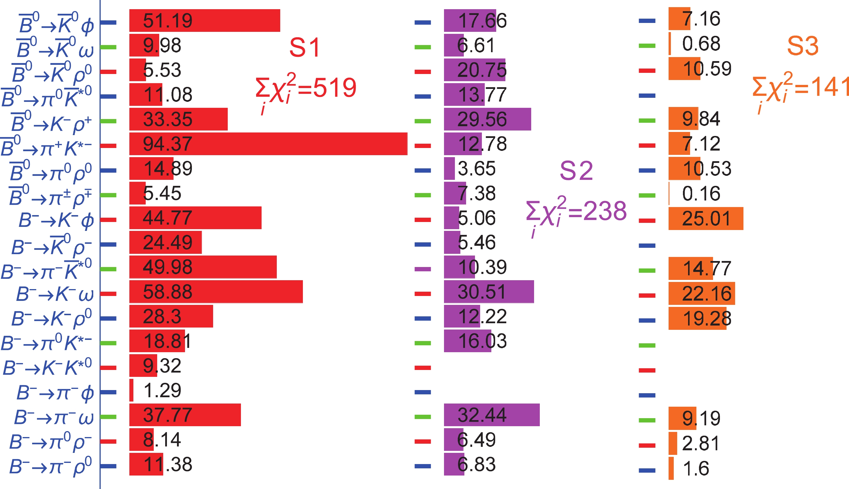
Figure 6.(color online)
$ {\chi}_{i}^{2} $ distribution of branching ratios for three scenarios, where the numbers in the bar charts denote the values of$ {\chi}_{i}^{2} $ for a specific process.mode $ B^{-} {\to} {\pi}^{-}{\rho}^{0} $ 

$ B^{-} {\to} {\pi}^{0}{\rho}^{-} $ 

$ B^{-} {\to} {\pi}^{-}{\omega} $ 

$ B^{-} {\to} {\pi}^{-}{\phi} $ 

data PDG $ 0.9{\pm}1.9 $ 

$ 2{\pm}11 $ 

$ -4{\pm}5 $ 

$ 9.8{\pm}51.1 $ 

S1 $ {\phi}_{B1} $ +

$ {\phi}_{B2} $ 

$ -24.00^{+ 0.61 + 1.16 }_{- 0.62 - 1.15 } $ 

$ 18.35^{+ 0.54 + 0.23 }_{- 0.53 - 0.24 } $ 

$ -1.67^{+ 0.01 + 0.26 }_{- 0.01 - 0.26 } $ 

$ 0 $ 

$ {\phi}_{B1} $ 

$ -29.49^{+ 0.81 + 1.25 }_{- 0.83 - 1.22 } $ 

$ 22.40^{+ 0.70 + 0.10 }_{- 0.68 - 0.11 } $ 

$ -4.36^{+ 0.02 + 0.18 }_{- 0.02 - 0.18 } $ 

$ 0 $ 

data BaBar $ 18{\pm}17 $ 

$ -1{\pm}13 $ 

$ -2{\pm}8 $ 

S2 $ {\phi}_{B1} $ +

$ {\phi}_{B2} $ 

$ -25.90^{+ 0.65 + 1.25 }_{- 0.66 - 1.23 } $ 

$ 19.98^{+ 0.56 + 0.26 }_{- 0.55 - 0.28 } $ 

$ -1.66^{+ 0.01 + 0.26 }_{- -0.00 - 0.26 } $ 

$ 0 $ 

$ {\phi}_{B1} $ 

$ -32.02^{+ 0.86 + 1.35 }_{- 0.88 - 1.32 } $ 

$ 24.52^{+ 0.73 + 0.13 }_{- 0.72 - 0.14 } $ 

$ -4.43^{+ 0.03 + 0.18 }_{- 0.02 - 0.17 } $ 

$ 0 $ 

data Belle $ 6{\pm}18 $ 

$ -2{\pm}9 $ 

S3 $ {\phi}_{B1} $ +

$ {\phi}_{B2} $ 

$ -22.20^{+ 0.58 + 1.08 }_{- 0.59 - 1.07 } $ 

$ 16.80^{+ 0.51 + 0.20 }_{- 0.50 - 0.21 } $ 

$ -1.68^{+ 0.00 + 0.26 }_{- 0.00 - 0.26 } $ 

$ 0 $ 

$ {\phi}_{B1} $ 

$ -27.09^{+ 0.77 + 1.15 }_{- 0.78 - 1.12 } $ 

$ 20.38^{+ 0.66 + 0.08 }_{- 0.65 - 0.09 } $ 

$ -4.28^{+ 0.03 + 0.18 }_{- 0.03 - 0.18 } $ 

$ 0 $ 

mode $ B^{-} {\to} K^{-}K^{{\ast}0} $ 

$ B^{-} {\to} K^{0}K^{{\ast}-} $ 

$ B^{-} {\to} {\pi}^{0}K^{{\ast}-} $ 

$ B^{-} {\to} K^{-}{\rho}^{0} $ 

data PDG $ 12.3{\pm}9.8 $ 

$ -39{\pm}21 $ 

$ 37{\pm}10 $ 

S1 $ {\phi}_{B1} $ +

$ {\phi}_{B2} $ 

$ 15.16^{+ 0.34 + 0.70 }_{- 0.34 - 0.58 } $ 

$ -25.13^{+ 2.03 + 13.90 }_{- 1.99 - 7.02 } $ 

$ -21.17^{+ 0.82 + 0.16 }_{- 0.84 - 0.15 } $ 

$ 82.79^{+ 1.30 + 3.37 }_{- 1.32 - 5.16 } $ 

$ {\phi}_{B1} $ 

$ 19.60^{+ 0.50 + 1.29 }_{- 0.51 - 1.03 } $ 

$ -11.19^{+ 1.82 + 7.91 }_{- 1.77 - 4.25 } $ 

$ -24.32^{+ 1.00 + 0.00 }_{- 1.02 - 0.01 } $ 

$ 78.05^{+ 1.52 + 0.57 }_{- 1.53 - 2.24 } $ 

data BaBar $ -52{\pm}15 $ 

$ 44{\pm}17 $ 

S2 $ {\phi}_{B1} $ +

$ {\phi}_{B2} $ 

$ 16.19^{+ 0.37 + 0.74 }_{- 0.35 - 0.60 } $ 

$ -19.01^{+ 2.03 + 13.91 }_{- 2.05 - 8.18 } $ 

$ -23.76^{+ 0.89 + 0.15 }_{- 0.91 - 0.14 } $ 

$ 78.79^{+ 1.35 + 3.20 }_{- 1.36 - 4.65 } $ 

$ {\phi}_{B1} $ 

$ 21.14^{+ 0.54 + 1.39 }_{- 0.52 - 1.09 } $ 

$ -5.72^{+ 1.82 + 8.30 }_{- 1.83 - 5.14 } $ 

$ -27.46^{+ 1.07 + 0.04 }_{- 1.09 - 0.05 } $ 

$ 73.45^{+ 1.54 + 0.72 }_{- 1.54 - 2.04 } $ 

data Belle $ 30{\pm}16 $ 

S3 $ {\phi}_{B1} $ +

$ {\phi}_{B2} $ 

$ 14.18^{+ 0.32 + 0.68 }_{- 0.31 - 0.55 } $ 

$ -31.01^{+ 1.93 + 13.31 }_{- 1.86 - 5.46 } $ 

$ -18.78^{+ 0.75 + 0.16 }_{- 0.77 - 0.15 } $ 

$ 86.60^{+ 1.20 + 3.42 }_{- 1.24 - 5.63 } $ 

$ {\phi}_{B1} $ 

$ 18.12^{+ 0.48 + 1.22 }_{- 0.47 - 0.96 } $ 

$ -16.43^{+ 1.73 + 7.11 }_{- 1.66 - 3.10 } $ 

$ -21.41^{+ 0.92 + 0.04 }_{- 0.95 - 0.04 } $ 

$ 82.55^{+ 1.45 + 0.28 }_{- 1.48 - 2.37 } $ 

mode $ B^{-} {\to} K^{-}{\omega} $ 

$ B^{-} {\to} {\pi}^{-}\overline{K}^{{\ast}0} $ 

$ B^{-} {\to} \overline{K}^{0}{\rho}^{-} $ 

$ B^{-} {\to} K^{-}{\phi} $ 

data PDG $ -2{\pm}4 $ 

$ -4{\pm}9 $ 

$ -3{\pm}15 $ 

$ 2.4{\pm}2.8 $ 

S1 $ {\phi}_{B1} $ +

$ {\phi}_{B2} $ 

$ 20.64^{+ 0.37 + 1.48 }_{- 0.38 - 1.06 } $ 

$ -1.13^{+ 0.03 + 0.03 }_{- 0.03 - 0.03 } $ 

$ 0.03^{+ 0.09 + 0.55 }_{- 0.09 - 0.64 } $ 

$ -0.55^{+ 0.01 + 0.02 }_{- 0.01 - 0.03 } $ 

$ {\phi}_{B1} $ 

$ 22.70^{+ 0.32 + 2.07 }_{- 0.33 - 1.50 } $ 

$ -1.48^{+ 0.05 + 0.05 }_{- 0.05 - 0.06 } $ 

$ -0.12^{+ 0.09 + 0.36 }_{- 0.08 - 0.42 } $ 

$ -0.69^{+ 0.02 + 0.04 }_{- 0.02 - 0.06 } $ 

data BaBar $ -1{\pm}7 $ 

$ -12{\pm}25 $ 

$ 21{\pm}31 $ 

$ 12.8{\pm}4.6 $ 

S2 $ {\phi}_{B1} $ +

$ {\phi}_{B2} $ 

$ 21.75^{+ 0.35 + 1.42 }_{- 0.36 - 1.01 } $ 

$ -1.23^{+ 0.03 + 0.03 }_{- 0.03 - 0.03 } $ 

$ -0.22^{+ 0.08 + 0.51 }_{- 0.07 - 0.56 } $ 

$ -0.59^{+ 0.01 + 0.02 }_{- 0.02 - 0.03 } $ 

$ {\phi}_{B1} $ 

$ 23.61^{+ 0.27 + 1.99 }_{- 0.29 - 1.44 } $ 

$ -1.63^{+ 0.05 + 0.06 }_{- 0.05 - 0.06 } $ 

$ -0.36^{+ 0.08 + 0.34 }_{- 0.07 - 0.38 } $ 

$ -0.76^{+ 0.02 + 0.04 }_{- 0.02 - 0.06 } $ 

data Belle $ -3{\pm}4 $ 

$ -14.9{\pm}6.8 $ 

$ 1{\pm}13 $ 

S3 $ {\phi}_{B1} $ +

$ {\phi}_{B2} $ 

$ 19.49^{+ 0.39 + 1.53 }_{- 0.40 - 1.09 } $ 

$ -1.04^{+ 0.03 + 0.02 }_{- 0.03 - 0.03 } $ 

$ 0.30^{+ 0.10 + 0.58 }_{- 0.10 - 0.71 } $ 

$ -0.51^{+ 0.01 + 0.02 }_{- 0.01 - 0.03 } $ 

$ {\phi}_{B1} $ 

$ 21.66^{+ 0.36 + 2.13 }_{- 0.38 - 1.53 } $ 

$ -1.34^{+ 0.04 + 0.05 }_{- 0.04 - 0.05 } $ 

$ 0.14^{+ 0.09 + 0.37 }_{- 0.09 - 0.47 } $ 

$ -0.64^{+ 0.02 + 0.04 }_{- 0.02 - 0.05 } $ 

Table 6.Direct
$C P$ -violating asymmetries ($ {\cal A}_{CP} $ , in the unit of percentage) for$ B_{u} {\to} PV $ decays. Other legends are the same as those ofTable 3.$ {\cal A}_{CP} $ 

mode $ \overline{B}^{0} {\to} {\pi}^{+}{\rho}^{-} $ 

$ \overline{B}^{0} {\to} {\pi}^{-}{\rho}^{+} $ 

$ \overline{B}^{0} {\to} {\pi}^{+}K^{{\ast}-} $ 

$ \overline{B}^{0} {\to} K^{-}{\rho}^{+} $ 

data PDG $ 13{\pm}6 $ 

$ -8{\pm}8 $ 

$ -27{\pm}4 $ 

$ 20{\pm}11 $ 

S1 $ {\phi}_{B1} $ +

$ {\phi}_{B2} $ 

$ 4.04^{+ 0.27 + 0.77 }_{- 0.26 - 0.80 } $ 

$ -19.80^{+ 0.35 + 0.18 }_{- 0.36 - 0.13 } $ 

$ -31.04^{+ 1.13 + 0.29 }_{- 1.15 - 0.33 } $ 

$ 86.31^{+ 0.61 + 2.50 }_{- 0.71 - 4.95 } $ 

$ {\phi}_{B1} $ 

$ 7.20^{+ 0.37 + 0.76 }_{- 0.36 - 0.80 } $ 

$ -22.88^{+ 0.48 + 0.26 }_{- 0.48 - 0.18 } $ 

$ -35.44^{+ 1.28 + 0.64 }_{- 1.29 - 0.74 } $ 

$ 74.34^{+ 0.83 + 3.15 }_{- 0.92 - 4.75 } $ 

data BaBar $ 9{\pm}7 $ 

$ -12{\pm}9 $ 

$ -29{\pm}11 $ 

$ 20{\pm}12 $ 

S2 $ {\phi}_{B1} $ +

$ {\phi}_{B2} $ 

$ 4.87^{+ 0.29 + 0.77 }_{- 0.28 - 0.81 } $ 

$ -20.91^{+ 0.38 + 0.12 }_{- 0.38 - 0.06 } $ 

$ -34.56^{+ 1.19 + 0.36 }_{- 1.21 - 0.40 } $ 

$ 83.91^{+ 0.89 + 1.48 }_{- 0.97 - 3.71 } $ 

$ {\phi}_{B1} $ 

$ 8.33^{+ 0.39 + 0.76 }_{- 0.39 - 0.80 } $ 

$ -24.36^{+ 0.51 + 0.18 }_{- 0.51 - 0.10 } $ 

$ -39.34^{+ 1.30 + 0.75 }_{- 1.30 - 0.85 } $ 

$ 71.37^{+ 1.06 + 2.15 }_{- 1.13 - 3.61 } $ 

data Belle $ 21{\pm}9 $ 

$ 8{\pm}19 $ 

$ -21{\pm}13 $ 

$ 22{\pm}24 $ 

S3 $ {\phi}_{B1} $ +

$ {\phi}_{B2} $ 

$ 3.27^{+ 0.25 + 0.76 }_{- 0.24 - 0.79 } $ 

$ -18.77^{+ 0.33 + 0.23 }_{- 0.34 - 0.19 } $ 

$ -27.72^{+ 1.06 + 0.24 }_{- 1.09 - 0.27 } $ 

$ 87.84^{+ 0.29 + 3.77 }_{- 0.40 - 6.31 } $ 

$ {\phi}_{B1} $ 

$ 6.14^{+ 0.34 + 0.75 }_{- 0.33 - 0.80 } $ 

$ -21.48^{+ 0.45 + 0.33 }_{- 0.46 - 0.26 } $ 

$ -31.64^{+ 1.23 + 0.55 }_{- 1.25 - 0.63 } $ 

$ 76.57^{+ 0.55 + 4.41 }_{- 0.65 - 6.03 } $ 

$ {\cal A}_{CP} $ 

mode $ \overline{B}^{0} {\to} {\pi}^{0}\overline{K}^{{\ast}0} $ 

$ \overline{B}^{0} {\to} \overline{K}^{0}{\rho}^{0} $ 

$ \overline{B}^{0} {\to} \overline{K}^{0}{\omega} $ 

$ \overline{B}^{0} {\to} \overline{K}^{0}{\phi} $ 

data PDG $ -15{\pm}13 $ 

$ -4{\pm}20 $ 

$ 0{\pm}40 $ 

$ 1{\pm}14 $ 

S1 $ {\phi}_{B1} $ +

$ {\phi}_{B2} $ 

$ -0.47^{+ 0.09 + 0.01 }_{- 0.08 - 0.01 } $ 

$ -5.47^{+ 0.16 + 1.72 }_{- 0.15 - 2.25 } $ 

$ 3.12^{+ 0.04 + 0.35 }_{- 0.04 - 0.29 } $ 

$ 0 $ 

$ {\phi}_{B1} $ 

$ -1.33^{+ 0.12 + 0.03 }_{- 0.10 - 0.02 } $ 

$ -6.57^{+ 0.20 + 1.80 }_{- 0.19 - 2.27 } $ 

$ 4.58^{+ 0.05 + 0.45 }_{- 0.05 - 0.35 } $ 

$ 0 $ 

data BaBar $ -15{\pm}13 $ 

$ -5{\pm}28 $ 

$ -52{\pm}22 $ 

$ 5{\pm}19 $ 

S2 $ {\phi}_{B1} $ +

$ {\phi}_{B2} $ 

$ -0.20^{+ 0.10 + 0.01 }_{- 0.10 - 0.01 } $ 

$ -5.88^{+ 0.12 + 1.65 }_{- 0.11 - 2.03 } $ 

$ 3.23^{+ 0.03 + 0.35 }_{- 0.03 - 0.29 } $ 

$ 0 $ 

$ {\phi}_{B1} $ 

$ -0.96^{+ 0.14 + 0.02 }_{- 0.13 - 0.01 } $ 

$ -7.08^{+ 0.15 + 1.69 }_{- 0.14 - 2.02 } $ 

$ 4.71^{+ 0.04 + 0.44 }_{- 0.04 - 0.34 } $ 

$ 0 $ 

data Belle $ -3{\pm}28 $ 

$ 36{\pm}20 $ 

$ -4{\pm}22 $ 

S3 $ {\phi}_{B1} $ +

$ {\phi}_{B2} $ 

$ -0.69^{+ 0.07 + 0.03 }_{- 0.06 - 0.03 } $ 

$ -4.97^{+ 0.19 + 1.75 }_{- 0.18 - 2.42 } $ 

$ 3.00^{+ 0.04 + 0.36 }_{- 0.04 - 0.29 } $ 

$ 0 $ 

$ {\phi}_{B1} $ 

$ -1.62^{+ 0.09 + 0.06 }_{- 0.08 - 0.06 } $ 

$ -5.93^{+ 0.24 + 1.86 }_{- 0.23 - 2.48 } $ 

$ 4.41^{+ 0.06 + 0.46 }_{- 0.06 - 0.36 } $ 

$ 0 $ 

mode $ \overline{B}^{0} {\to} {\pi}^{0}{\rho}^{0} $ 

$ \overline{B}^{0} {\to} {\pi}^{0}{\omega} $ 

$ C_{f} $ 

$ S_{f} $ 

$ C_{f} $ 

$ S_{f} $ 

data PDG $ 27{\pm}24 $ 

$ -23{\pm}34 $ 

S1 $ {\phi}_{B1} $ +

$ {\phi}_{B2} $ 

$ -0.04^{+ 0.14 + 0.31 }_{- 0.21 - 0.50 } $ 

$ -89.75^{+ 0.46 + 2.11 }_{- 0.45 - 1.82 } $ 

$ -67.36^{+ 1.06 + 0.75 }_{- 1.05 - 0.73 } $ 

$ 24.00^{+ 0.40 + 1.86 }_{- 0.40 - 1.78 } $ 

$ {\phi}_{B1} $ 

$ -22.82^{+ 0.03 + 0.11 }_{- 0.06 - 0.22 } $ 

$ -74.39^{+ 0.50 + 3.22 }_{- 0.49 - 2.90 } $ 

$ -66.52^{+ 1.05 + 0.33 }_{- 1.04 - 0.32 } $ 

$ 39.32^{+ 0.41 + 0.97 }_{- 0.42 - 0.89 } $ 

data BaBar $ 19{\pm}27 $ 

$ -37{\pm}39 $ 

S2 $ {\phi}_{B1} $ +

$ {\phi}_{B2} $ 

$ 0.49^{+ 0.21 + 0.26 }_{- 0.18 - 0.42 } $ 

$ -88.39^{+ 0.46 + 2.27 }_{- 0.45 - 1.96 } $ 

$ -70.49^{+ 1.05 + 0.82 }_{- 1.03 - 0.79 } $ 

$ 25.15^{+ 0.32 + 1.79 }_{- 0.38 - 1.74 } $ 

$ {\phi}_{B1} $ 

$ -22.65^{+ 0.09 + 0.10 }_{- 0.08 - 0.20 } $ 

$ -73.00^{+ 0.42 + 3.28 }_{- 0.43 - 2.98 } $ 

$ -69.62^{+ 1.03 + 0.36 }_{- 1.03 - 0.36 } $ 

$ 40.43^{+ 0.28 + 0.85 }_{- 0.35 - 0.79 } $ 

data Belle $ 49{\pm}46 $ 

$ 17{\pm}67 $ 

S3 $ {\phi}_{B1} $ +

$ {\phi}_{B2} $ 

$ -0.57^{+ 0.13 + 0.43 }_{- 0.11 - 0.57 } $ 

$ -91.10^{+ 0.46 + 1.94 }_{- 0.45 - 1.64 } $ 

$ -64.23^{+ 1.05 + 0.67 }_{- 1.03 - 0.65 } $ 

$ 22.69^{+ 0.46 + 1.91 }_{- 0.46 - 1.84 } $ 

$ {\phi}_{B1} $ 

$ -22.90^{+ 0.05 + 0.15 }_{- 0.01 - 0.23 } $ 

$ -76.00^{+ 0.58 + 3.11 }_{- 0.60 - 2.78 } $ 

$ -63.47^{+ 1.00 + 0.27 }_{- 1.00 - 0.27 } $ 

$ 37.90^{+ 0.53 + 1.07 }_{- 0.55 - 1.00 } $ 

Table 7.
$C P$ -violating asymmetries (in the unit of percentage) for$ B_{d} $ decays. Other legends are the same as those ofTable 3.$ {\pi}^{+}{\rho}^{-} $ ,

$ {\pi}^{-}{\rho}^{+} $ 

$ a_{{\epsilon}^{\prime}} $ 

$ a_{{\epsilon}+{\epsilon}^{\prime}} $ 

$ \bar{a}_{{\epsilon}^{\prime}} $ 

$ \bar{a}_{{\epsilon}+{\epsilon}^{\prime}} $ 

data PDG $ -3{\pm}7 $ 

$ 5{\pm}7 $ 

S1 $ {\phi}_{B1} $ +

$ {\phi}_{B2} $ 

$ -19.23^{+ 0.34 + 3.24 }_{- 0.34 - 3.06 } $ 

$ 9.05^{+ 0.03 + 1.00 }_{- 0.03 - 1.00 } $ 

$ 27.32^{+ 0.22 + 3.26 }_{- 0.22 - 3.46 } $ 

$ 12.71^{+ 0.09 + 1.36 }_{- 0.09 - 1.36 } $ 

$ {\phi}_{B1} $ 

$ -22.66^{+ 0.38 + 4.00 }_{- 0.38 - 3.72 } $ 

$ 9.78^{+ 0.03 + 1.14 }_{- 0.03 - 1.15 } $ 

$ 32.52^{+ 0.21 + 4.04 }_{- 0.20 - 4.37 } $ 

$ 9.60^{+ 0.04 + 1.60 }_{- 0.04 - 1.59 } $ 

data BaBar $ 1.6{\pm}6.9 $ 

$ 5.3{\pm}8.8 $ 

S2 $ {\phi}_{B1} $ +

$ {\phi}_{B2} $ 

$ -18.25^{+ 0.31 + 3.18 }_{- 0.32 - 3.00 } $ 

$ 8.97^{+ 0.02 + 0.96 }_{- 0.03 - 0.96 } $ 

$ 26.71^{+ 0.19 + 3.24 }_{- 0.19 - 3.43 } $ 

$ 12.99^{+ 0.10 + 1.33 }_{- 0.10 - 1.34 } $ 

$ {\phi}_{B1} $ 

$ -21.56^{+ 0.34 + 3.95 }_{- 0.36 - 3.68 } $ 

$ 9.88^{+ 0.03 + 1.09 }_{- 0.04 - 1.09 } $ 

$ 31.97^{+ 0.17 + 4.05 }_{- 0.16 - 4.37 } $ 

$ 9.70^{+ 0.04 + 1.57 }_{- 0.04 - 1.57 } $ 

data Belle $ -13{\pm}10 $ 

$ 6{\pm}14 $ 

S3 $ {\phi}_{B1} $ +

$ {\phi}_{B2} $ 

$ -20.29^{+ 0.36 + 3.30 }_{- 0.38 - 3.11 } $ 

$ 9.13^{+ 0.03 + 1.04 }_{- 0.03 - 1.04 } $ 

$ 28.03^{+ 0.26 + 3.28 }_{- 0.25 - 3.49 } $ 

$ 12.44^{+ 0.09 + 1.38 }_{- 0.09 - 1.38 } $ 

$ {\phi}_{B1} $ 

$ -23.84^{+ 0.41 + 4.05 }_{- 0.42 - 3.75 } $ 

$ 9.68^{+ 0.04 + 1.20 }_{- 0.03 - 1.19 } $ 

$ 33.19^{+ 0.25 + 4.02 }_{- 0.23 - 4.36 } $ 

$ 9.50^{+ 0.03 + 1.62 }_{- 0.04 - 1.61 } $ 

$ \overline{K}^{0}K^{{\ast}0} $ ,

$ K^{0}\overline{K}^{{\ast}0} $ 

$ a_{{\epsilon}^{\prime}} $ 

$ a_{{\epsilon}+{\epsilon}^{\prime}} $ 

$ \bar{a}_{{\epsilon}^{\prime}} $ 

$ \bar{a}_{{\epsilon}+{\epsilon}^{\prime}} $ 

data PDG S1 $ {\phi}_{B1} $ +

$ {\phi}_{B2} $ 

$ -76.49^{+ 1.10 + 1.14 }_{- 1.05 - 0.53 } $ 

$ 58.96^{+ 1.43 + 4.66 }_{- 1.42 - 4.44 } $ 

$ 76.49^{+ 1.05 + 0.53 }_{- 1.10 - 1.14 } $ 

$ -58.96^{+ 1.42 + 4.44 }_{- 1.43 - 4.66 } $ 

$ {\phi}_{B1} $ 

$ -64.09^{+ 1.43 + 1.69 }_{- 1.37 - 0.24 } $ 

$ 61.42^{+ 1.34 + 6.32 }_{- 1.34 - 5.61 } $ 

$ 64.09^{+ 1.37 + 0.24 }_{- 1.43 - 1.69 } $ 

$ -61.42^{+ 1.34 + 5.61 }_{- 1.34 - 6.32 } $ 

data BaBar S2 $ {\phi}_{B1} $ +

$ {\phi}_{B2} $ 

$ -73.04^{+ 1.25 + 1.01 }_{- 1.20 - 0.69 } $ 

$ 63.22^{+ 1.40 + 4.78 }_{- 1.41 - 4.61 } $ 

$ 73.04^{+ 1.20 + 0.69 }_{- 1.25 - 1.01 } $ 

$ -63.22^{+ 1.41 + 4.61 }_{- 1.40 - 4.78 } $ 

$ {\phi}_{B1} $ 

$ -59.64^{+ 1.58 + 1.11 }_{- 1.53 - 0.43 } $ 

$ 65.34^{+ 1.24 + 6.41 }_{- 1.27 - 5.78 } $ 

$ 59.64^{+ 1.53 + 0.43 }_{- 1.58 - 1.11 } $ 

$ -65.34^{+ 1.27 + 5.78 }_{- 1.24 - 6.41 } $ 

data Belle S3 $ {\phi}_{B1} $ +

$ {\phi}_{B2} $ 

$ -79.48^{+ 0.95 + 1.56 }_{- 0.90 - 0.05 } $ 

$ 54.71^{+ 1.41 + 4.50 }_{- 1.40 - 4.25 } $ 

$ 79.48^{+ 0.90 + 0.05 }_{- 0.95 - 1.56 } $ 

$ -54.71^{+ 1.40 + 4.25 }_{- 1.41 - 4.50 } $ 

$ {\phi}_{B1} $ 

$ -68.05^{+ 1.27 + 2.23 }_{- 1.22 - 0.89 } $ 

$ 57.33^{+ 1.37 + 6.13 }_{- 1.39 - 5.39 } $ 

$ 68.05^{+ 1.22 + 0.89 }_{- 1.27 - 2.23 } $ 

$ -57.33^{+ 1.39 + 5.39 }_{- 1.37 - 6.13 } $ 

$ K^{+}K^{{\ast}-} $ ,

$ K^{-}K^{{\ast}+} $ 

$ a_{{\epsilon}^{\prime}} $ 

$ a_{{\epsilon}+{\epsilon}^{\prime}} $ 

$ \bar{a}_{{\epsilon}^{\prime}} $ 

$ \bar{a}_{{\epsilon}+{\epsilon}^{\prime}} $ 

data PDG S1 $ {\phi}_{B1} $ +

$ {\phi}_{B2} $ 

$ -14.02^{+ 0.79 + 0.86 }_{- 0.71 - 0.95 } $ 

$ -38.60^{+ -0.01 + 0.60 }_{- 0.03 - 0.62 } $ 

$ 67.26^{+ 0.34 + 0.17 }_{- 0.32 - 0.10 } $ 

$ -11.47^{+ 0.44 + 0.69 }_{- 0.47 - 0.69 } $ 

$ {\phi}_{B1} $ 

$ 11.39^{+ 0.07 + 0.17 }_{- -0.05 - 0.23 } $ 

$ -41.60^{+ 0.20 + 0.63 }_{- 0.17 - 0.56 } $ 

$ 27.65^{+ 0.89 + 0.42 }_{- 0.88 - 0.38 } $ 

$ -1.97^{+ 0.05 + 1.45 }_{- 0.15 - 1.41 } $ 

data BaBar S2 $ {\phi}_{B1} $ +

$ {\phi}_{B2} $ 

$ -16.09^{+ 0.63 + 0.79 }_{- 0.72 - 0.87 } $ 

$ -38.54^{+ 0.05 + 0.58 }_{- 0.04 - 0.63 } $ 

$ 66.24^{+ 0.40 + 0.15 }_{- 0.33 - 0.11 } $ 

$ -10.14^{+ 0.46 + 0.73 }_{- 0.44 - 0.71 } $ 

$ {\phi}_{B1} $ 

$ 11.56^{+ -0.01 + 0.07 }_{- 0.12 - 0.14 } $ 

$ -40.90^{+ 0.25 + 0.63 }_{- 0.27 - 0.63 } $ 

$ 25.04^{+ 0.94 + 0.45 }_{- 0.86 - 0.46 } $ 

$ -1.80^{+ 0.07 + 1.47 }_{- 0.04 - 1.38 } $ 

data Belle S3 $ {\phi}_{B1} $ +

$ {\phi}_{B2} $ 

$ -11.66^{+ 0.89 + 0.93 }_{- 0.81 - 1.03 } $ 

$ -38.60^{+ -0.02 + 0.63 }_{- 0.04 - 0.66 } $ 

$ 68.33^{+ 0.31 + 0.13 }_{- 0.38 - 0.12 } $ 

$ -12.84^{+ 0.48 + 0.69 }_{- 0.50 - 0.64 } $ 

$ {\phi}_{B1} $ 

$ 11.38^{+ 0.05 + 0.25 }_{- -0.04 - 0.29 } $ 

$ -42.02^{+ 0.09 + 0.67 }_{- 0.07 - 0.62 } $ 

$ 30.49^{+ 0.95 + 0.32 }_{- 1.03 - 0.34 } $ 

$ -2.33^{+ 0.14 + 1.48 }_{- 0.19 - 1.35 } $ 

Table 8.
$C P$ -violating asymmetries (in the unit of percentage) for Case 3$ B_{d} $ decays. Other legends are the same as those ofTable 3.(1) As shown inTables 3and4, except for the
$ B^{-} {\to} \overline{K}^{0}{\rho}^{-} $ and$ K^{0}K^{{\ast}-} $ decays, the contributions from theBmesonic WFs$ {\phi}_{B2} $ can enhance the branching ratios compared with those from$ {\phi}_{B1} $ . The contributions from$ {\phi}_{B2} $ to the branching ratios are approximately$ 30\ $ % and sometimes more, except for the$ \overline{B} {\to} K{\rho} $ ,$ K{\omega} $ ,$ {\pi}{\phi} $ ,$ {\pi}^{0}{\rho}^{0} $ ,$ K^{0}K^{{\ast}-} $ , and$ K^{-}K^{{\ast}+} $ decays. In addition, as shown inTables 5, various results are obtained with the PQCD approach at the LO and NLO levels. The previous PQCD studies in Refs. [50,53,55] have shown that the NLO contributions can sometimes enhance and sometimes lessen the LO branching ratios. The shares from$ {\phi}_{B2} $ to the branching ratios are comparable to the module of the shares from the NLO contributions. Taking the branching ratios for the$ B^{-} {\to} {\pi}^{-}{\rho}^{0} $ ($ K^{-}K^{{\ast}0} $ ) decays as an example, the shares from$ {\phi}_{B2} $ are approximately$ 37 $ % ($ 30 $ %), and the shares from the NLO contributions are approximately$ 40 $ % [50] ($ 24 $ % [53]). On the whole, considerably more effort is required to further improve the agreement between the theoretical results and data.(2) As shown inTables 6and7, the participation of the WFs
$ {\phi}_{B2} $ results in a small reduction in the direct$C P$ asymmetries, except for the$ \overline{B} {\to} K^{-}{\rho} $ and$ K^{0}K^{{\ast}-} $ decays. As is well known, the theoretical results of the$C P$ asymmetries are highly sensitive to the strong phases. Therefore, it is essential to obtain the strong phases as accurately as possible. There are numerous sources of strong phases, such as the higher order radiative corrections to HMEs and final state interactions. In this paper,$C P$ asymmetries are calculated at the LO order, and many factors that might affect these asymmetries are not carefully considered owing to our inadequate comprehension. For instance, there are still many theoretical and experimental discrepancies on the branching ratios. Therefore, our$C P$ asymmetry estimations inTables 6,7, and8cannot be taken too literally. Moreover, it is assumed that the current precision of most measurements of$C P$ asymmetries is too low to impose helpful constraints. Given their theoretical and experimental research status,$C P$ asymmetries are not considered in the fit with Eq. (55). In addition, it is shown in the amplitudes of Eq. (A4), Eq. (A19), and Eq. (A25) that tree amplitudes are absent and only the penguin contributions participate. These facts result in unavailable weak phase differences, which are an essential ingredient of direct$C P$ asymmetries. Therefore, it is not surprising that the theoretical expectations of the direct$C P$ asymmetries for the$ B^{-} {\to} {\pi}^{-}{\phi} $ and$ \overline{B}^{0} {\to} {\pi}^{0}{\phi} $ ,$ \overline{K}^{0}{\phi} $ decays are exactly zero. For$ \overline{B}^{0} {\to} \overline{K}^{0}K^{{\ast}0} + K^{0}\overline{K}^{{\ast}0} $ decays, which are induced by the pure penguin amplitudes in Eq. (A17) and Eq. (A18), the parameters$ {\lambda}_{f} $ of Eq. (53) and$ \bar{\lambda}_{f} $ of Eq. (54) contain only strong phase information. The measurements of the observables$ a_{{\epsilon}^{\prime}} = -\bar{a}_{{\epsilon}^{\prime}} $ and$a_{{\epsilon}+{\epsilon}^{\prime}} = -\bar{a}_{{\epsilon}+{\epsilon}^{\prime}}$ would be helpful for testing our understanding on the strong interactions in nonleptonicBmeson weak decays.(3) It is clear inFig. 6that for S1, the goodness of fit between the PDG group data and PQCD results is still far from satisfactory. Among the 19
$ B {\to} PV $ decays, there are only four decay modes with$ {\chi}_{i}^{2} < 9 $ , which indicates that the theoretical results on the branching ratios for the$ B^{-} {\to} {\pi}^{0}{\rho}^{-} $ ,$ {\pi}^{-}{\phi} $ ,$ \overline{B}^{0} {\to} {\pi}^{\pm}{\rho}^{\mp} $ , and$ \overline{K}^{0}{\rho}^{0} $ decays agree with the PDG data within three standard experimental errors. The minimal$ {\chi}_{i}^{2} {\approx} 1.3 $ is obtained for the$ B^{-} {\to} {\pi}^{-}{\phi} $ decay, where the relative fitting error is significantly large and can reach up to approximately$ 47 $ %. (Note: There is a general and conventional consensus in elementary particle physics that a signal or event with a statistic significance of less than$ 3\,{\sigma} $ , more than$ 3\,{\sigma} $ , and more than$ 5\,{\sigma} $ are respectively known as a hint (or an indication), an evidence, and a discovery (or an observation or a confirmation), usually with a relative error greater than$33.3$ %, lower than$ 33.3 $ %, and lower than$ 20 $ %.) There are eight decay modes with$ {\chi}_{i}^{2} > 25 $ , which suggests that the discrepancies between theoretical calculations and the data are larger than five standard experimental errors, and the theoretical results on the$ B^{-} {\to} {\pi}^{-}{\omega} $ ,$ K^{-}{\rho}^{0} $ ,$ K^{-}{\omega} $ ,$ K^{-}{\phi} $ ,$ {\pi}^{-}\overline{K}^{{\ast}0} $ and$ \overline{B}^{0} {\to} {\pi}^{+}K^{{\ast}-} $ ,$ K^{-}{\rho}^{+} $ ,$ \overline{K}^{0}{\phi} $ decays fail to provide a satisfactory explanation for the PDG data. The maximal$ {\chi}_{i}^{2} {\approx} 94 $ is found for the$ \overline{B}^{0} {\to} {\pi}^{+}K^{{\ast}-} $ decay, where the relative fitting error is significantly small at approximately$ 5\ $ %. It should be noted that the disagreement about the$ \overline{B}^{0} {\to} {\pi}^{+}K^{{\ast}-} $ decay has been reported by previous PQCD studies in which only the$ {\phi}_{B1} $ contributions were considered, for example,$ {\chi}_{i}^{2} {\approx} 36 $ ($ 14 $ ) with the LO (NLO) contributions [55] and$ {\chi}_{i}^{2} {\approx} 41 $ with the recent global analysis ofBdecays [54] at the LO level. For S2 (S3), there are seven (six) decay modes with$ {\chi}_{i}^{2} < 9 $ .$ B^{-} {\to} K^{-}{\phi} $ is the only decay with$ {\chi}_{i}^{2} $ just above$ 25 $ in S3. In both scenarios, the$ B^{-} {\to} {\pi}^{0}{\rho}^{-} $ and$ \overline{B}^{0} {\to} {\pi}^{\pm}{\rho}^{\mp} $ decays have$ {\chi}_{i}^{2} < 9 $ at present.(4) As shown inFig. 6, there are four decays with
$ {\chi}_{i}^{2} {\ge} 50 $ in S1, including the$ B^{-} {\to} K^{-}{\omega} $ ,$ {\pi}^{-}\overline{K}^{{\ast}0} $ and$ \overline{B}^{0} {\to} {\pi}^{+}K^{{\ast}-} $ ,$ \overline{K}^{0}{\phi} $ decays. To further explore other possible underlying causes for the relatively larger$ {\chi}_{\rm min}^{2} $ for S1 besides the relatively smaller errors in the PDG data, the relations of the branching ratios versus the shape parameter$ {\omega}_{B} $ are shown inFig. 7. There are several clear and attractive phenomena evident inFig. 7. (i) Most of the branching ratios decrease with an increase in the parameter$ {\omega}_{B} $ . This situation is similar to that of form factors inFig. 3. It is easy to understand this phenomenon because decay amplitudes are usually proportional to form factors. (ii) The current PDG data on the$ B^{-} {\to} \overline{K}^{0}{\rho}^{-} $ ,$ K^{-}{\rho}^{0} $ and$ \overline{B}^{0} {\to} K^{-}{\rho}^{+} $ ,$ {\pi}^{0}{\rho}^{0} $ decays cannot be satisfactorily explained using the PQCD approach within$ 3\,{\sigma} $ regions, no matter which value is taken for the parameter within$ 0.3 $ GeV$ {\le} {\omega}_{B} {\le} 0.6 $ GeV. These four decays contribute a large$ {\chi}_{i}^{2} > 9 $ . In addition, the branching ratios of these four decays are insensitive to the parameter$ {\omega}_{B} $ . (iii) When the pseudoscalar pion meson is one of the final states, branching ratios change significantly with the parameter$ {\omega}_{B} $ , except for the above mentioned$ \overline{B}^{0} {\to} {\pi}^{0}{\rho}^{0} $ decay. A small$ {\omega}_{B} < 0.4 $ GeV is commonly favored by mostBdecays, except for the$ B^{-} {\to} {\pi}^{-}{\phi} $ decay. Although the PGD data opt for a large$ {\omega}_{B} $ for the$ B^{-} {\to} {\pi}^{-}{\phi} $ decay, the value of$ {\omega}_{B} = 0.4 $ GeV can also marginally meet the experimental$ 3\,{\sigma} $ constraints. The S1 parameter$ {\omega}_{B} = 0.46 $ GeV is somewhat large and should be decreased for$ B {\to} {\pi}V $ decays, which results in the extraordinarily large$ {\chi}_{i}^{2} {\approx} 38 $ ,$ 50 $ , and$ 94 $ corresponding respectively to the$ \overline{B} {\to} {\pi}^{-}{\omega} $ ,$ {\pi}^{-}\overline{K}^{{\ast}0} $ , and$ {\pi}^{+}\overline{K}^{{\ast}0} $ decays. (iv) When the pseudoscalar kaon meson is one of the final states, the PDG data impose inconsistent requirements on the parameter$ {\omega}_{B} $ , that is,$ {\omega}_{B} < 0.45 $ GeV for the$ \overline{B} {\to} \overline{K}{\omega} $ ,$ K^{-}K^{{\ast}0} $ decays, and$ {\omega}_{B} > 0.5 $ GeV for the$ \overline{B} {\to} \overline{K}{\phi} $ decays. The positive and negative deviations from$ {\omega}_{B} = 0.46 $ GeV facilitate$ {\chi}_{i}^{2} $ for the$ \overline{B} {\to} K^{-}{\omega} $ ,$ K^{-}{\phi} $ , and$ \overline{K}^{0}{\phi} $ decays to$ 59 $ ,$ 45 $ , and$ 51 $ , respectively. (v) The general conclusion about S1 is that, on the one hand, a relatively small$ {\omega}_{B} $ is favored by the$ \overline{B} {\to} \overline{K}{\omega} $ decays and most of the$ \overline{B} {\to} {\pi}V $ decays. On the other hand, a relatively large$ {\omega}_{B} $ is favored by the$ \overline{B} {\to} P{\phi} $ decays. Furthermore, the$ \overline{B} {\to} \overline{K}{\rho} $ decays are insensitive to changes in$ {\omega}_{B} $ .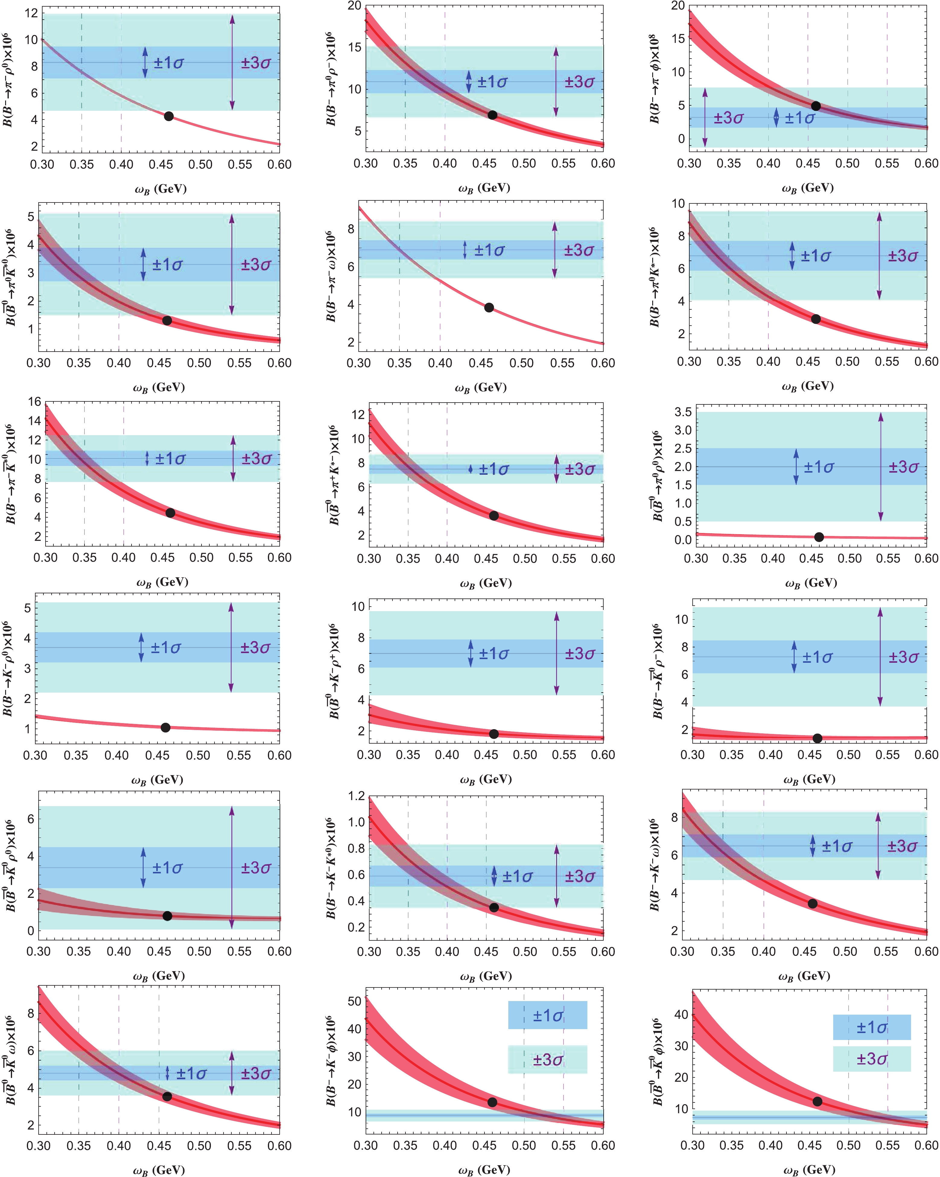
Figure 7.(color online) Branching ratios vs the shape parameter
$ {\omega}_{B} $ , where the relatively narrower (wider) horizontal bands denote the PGD data within$ {\pm}1\,{\sigma} $ ($ {\pm}3\,{\sigma} $ ) regions, the curves in red are the PQCD results, including contributions from$ {\phi}_{B2} $ , the curvy bands in pink denote the theoretical uncertainties from the chiral mass$ {\mu}_{P} = 1.4{\pm}0.1 $ GeV, and the points in black denote the S1 results.(5) As shown inTable 5, previous PQCD results without contributions from theBmesonic WFs
$ {\phi}_{B2} $ could also provide a satisfactory explanation for many of the$ B {\to} PV $ decays by choosing appropriate parameters, such as$ {\omega}_{B} $ . In other words, to some extent, the effects of$ {\phi}_{B2} $ on nonleptonicBdecays could be replaced by other scenarios of input parameters, which might be one reason why the contributions of$ {\phi}_{B2} $ were often not seriously considered in previous studies. To further illustrate the influences of$ {\phi}_{B2} $ on$ B {\to} PV $ decays, consistencies between the experimental data and PQCD results with different$ {\omega}_{B} $ are shown inFigs. 8and9. It is clear fromFig. 8that when contributions from theBmesonic WFs$ {\phi}_{B2} $ are not taken into account, the optimal parameter$ {\omega}_{B} $ and the minimum$ {\chi}^{2} $ corresponding to experimental data from the BaBar and Belle groups are, respectively,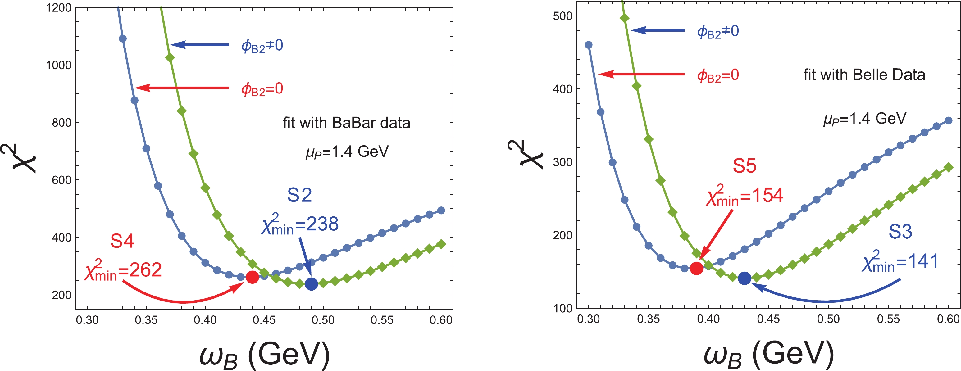
Figure 8.(color online) Distribution of
$ {\chi}^{2} $ versus the shape parameter$ {\omega}_{B} $ with and without the contributions of$ {\phi}_{B2} $ .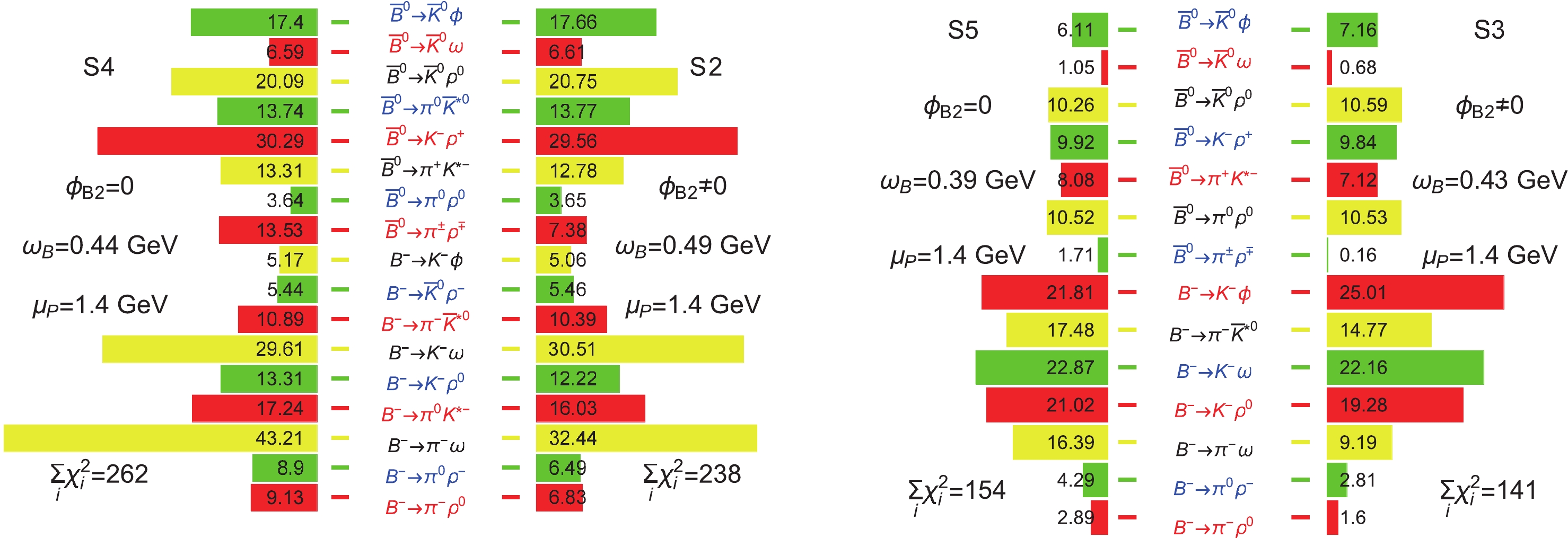
Figure 9.(color online)
$ {\chi}_{i}^{2} $ distribution of branching ratios with and without the contributions of$ {\phi}_{B2} $ , where the numbers in the bar charts denote the values of$ {\chi}_{i}^{2} $ for a specific process.● Scenario 4 (S4):
$ {\omega}_{B} = 0.44 $ GeV from BaBar data with$ {\chi}^{2}_{\rm min.} {\approx} 262 $ ,● Scenario 5 (S5):
$ {\omega}_{B} = 0.39 $ GeV from Belle data with$ {\chi}^{2}_{\rm min.} {\approx} 154 $ .The value of
$ {\omega}_{B} $ for S4 (S5) is less than that for S2 (S3). The value of$ {\chi}^{2}_{\rm min.} $ for S4 (S5) is larger than that for S2 (S3). As shown inFig. 9, (i) there are five decay modes with$ {\chi}^{2}_{i} < 9 $ for S4, which is fewer than the seven decay modes with$ {\chi}^{2}_{i} < 9 $ for S2. (ii) There are six same decay modes with$ {\chi}^{2}_{i} < 9 $ for both S3 and S5, including the$ B^{-} {\to} {\pi}^{-}{\rho}^{0} $ ,$ {\pi}^{0}{\rho}^{-} $ and$ \overline{B}^{0} {\to} {\pi}^{\pm}{\rho}^{\mp} $ ,$ {\pi}^{+}\overline{K}^{{\ast}-} $ ,$ \overline{K}^{0}{\omega} $ ,$ \overline{K}^{0}{\phi} $ decays. Among these six same decays, except for the$ \overline{B}^{0} {\to} \overline{K}^{0}{\phi} $ decay, the$ {\chi}^{2}_{i} $ of the other decays for S5 are larger than that for S3. A conclusion from the comparative analysis ofFigs. 8and9is that a more comprehensive agreement of branching ratios between the PQCD calculations and experimental data can be improved by the participation of theBmesonic WFs$ {\phi}_{B2} $ . -
In this study, inspired by the experimental prospects ofBmeson physics, we reinvestigate
$ B {\to} PV $ decays ($ P = {\pi} $ andK) at the LO order using the PQCD approach within the SM by considering theBmesonic WFs$ {\phi}_{B2} $ , which have been excluded in previous phenomenological studies. In the convolution integrals of the HMEs of nonleptonicBdecays, the WFs$ {\phi}_{B2} $ are involved in the emission amplitudes and nonfactorizable annihilation amplitudes. Contributions from$ {\phi}_{B2} $ can enhance the hadronic transition form factors$ F_{1}(0) $ and$ A_{0}(0) $ . The form factors are highly sensitive to the shape parameter$ {\omega}_{B} $ ofBmesonic WFs. By fitting the PQCD results with the branching ratios and experimental data using the minimum$ {\chi}^{2} $ method, it is found that the participation of$ {\phi}_{B2} $ is helpful for improving the comprehensive agreement between the PQCD calculations and experimental data. The shares of$ {\phi}_{B2} $ should be given due attention and studied meticulously for nonleptonicBdecays. When contributions from$ {\phi}_{B2} $ are considered, three optimal scenarios of the parameter$ {\omega}_{B} $ are found. The PQCD results on branching ratios and$C P$ asymmetries are updated with these three scenarios. It is found that in any one of these scenarios, the$ {\phi}_{B2} $ contributions can increase most branching ratios, except for the$ B^{-} {\to} K^{0}K^{{\ast}-} $ ,$ \overline{K}^{0}{\rho}^{-} $ decays. In contrast, these contributions can decrease most direct$C P$ asymmetries, except in the$ \overline{B} {\to} K^{-}{\rho} $ and$ K^{0}K^{{\ast}-} $ decays. However, it should be noted that there are still several discrepancies between the PQCD results and available data to a greater or lesser extent. More worthwhile endeavors on nonleptonicBdecays are required, experimentally and theoretically. From the experimental perspective, an increasing number of accurate measurement results are being produced within existing and future experiments. From the theoretical perspective, at the quark level, other possible mechanisms of the interactions and higher order corrections of scattering amplitudes are highly important; at the hadron level, some appropriate models for mesonic WFs including higher twist components are essential. -
Using the
$S U(3)$ flavor structure, a more concise and compact amplitude for the$ B {\to} PP $ ,$ PV $ decays is given by Eq. (12) in Ref. [54] with the PQCD approach. The analytical expressions are explicitly listed below.$ \begin{aligned}[b] {\cal A}(B_{u}^-{\to}{\pi}^-{\rho}^{0}) =& \frac{G_{\rm F}}{2}\, V_{ub}\,V_{ud}^{\ast}\, \big\{ a_{1}\, \big[ {\cal A}_{ab}^{LL}({\pi},{\rho}) + {\cal A}_{ef}^{LL}({\pi},{\rho}) - {\cal A}_{ef}^{LL}({\rho},{\pi}) \big] + a_{2}\, {\cal A}_{ab}^{LL}({\rho},{\pi}) + C_{2}\, \big[ {\cal A}_{cd}^{LL}({\pi},{\rho}) + {\cal A}_{gh}^{LL}({\pi},{\rho}) - {\cal A}_{gh}^{LL}({\rho},{\pi}) \big] \\ & + C_{1}\, {\cal A}_{cd}^{LL}({\rho},{\pi}) \big\} - \frac{G_{\rm F}}{2}\, V_{tb}\,V_{td}^{\ast}\, \big\{ (a_{4}+a_{10}) \, \big[ {\cal A}_{ab}^{LL}({\pi},{\rho}) + {\cal A}_{ef}^{LL}({\pi},{\rho}) - {\cal A}_{ef}^{LL}({\rho},{\pi}) \big] \\ & + (a_{6}+a_{8})\, \big[ {\cal A}_{ab}^{SP}({\pi},{\rho}) + {\cal A}_{ef}^{SP}({\pi},{\rho}) - {\cal A}_{ef}^{SP}({\rho},{\pi}) \big] - (a_{4} -\frac{3}{2}\,a_{7} - \frac{3}{2}\,a_{9} -\frac{1}{2}\,a_{10} ) \, {\cal A}_{ab}^{LL}({\rho},{\pi}) \\ & + (C_{3}+C_{9}) \, \big[ {\cal A}_{cd}^{LL}({\pi},{\rho}) + {\cal A}_{gh}^{LL}({\pi},{\rho}) - {\cal A}_{gh}^{LL}({\rho},{\pi}) \big] + (C_{5}+C_{7})\, \big[ {\cal A}_{cd}^{SP}({\pi},{\rho}) + {\cal A}_{gh}^{SP}({\pi},{\rho}) - {\cal A}_{gh}^{SP}({\rho},{\pi}) \big] \\ & - (C_{3} - \frac{3}{2}\,C_{10} -\frac{1}{2}\,C_{9} ) \, {\cal A}_{cd}^{LL}({\rho},{\pi}) + \frac{3}{2}\,C_{8}\, {\cal A}_{cd}^{LR}({\rho},{\pi}) - (C_{5}-\frac{1}{2}\,C_{7})\, {\cal A}_{cd}^{SP}({\rho},{\pi}) \big\} , \end{aligned} \tag{A1}$ 
$ \begin{aligned}[b] {\cal A}(B_{u}^-{\to}{\rho}^-{\pi}^{0}) =& \frac{G_{\rm F}}{2}\, V_{ub}\,V_{ud}^{\ast}\, \big\{ a_{1}\, \big[ {\cal A}_{ab}^{LL}({\rho},{\pi}) + {\cal A}_{ef}^{LL}({\rho},{\pi}) - {\cal A}_{ef}^{LL}({\pi},{\rho}) \big] + a_{2}\, {\cal A}_{ab}^{LL}({\pi},{\rho}) + C_{2}\, \big[ {\cal A}_{cd}^{LL}({\rho},{\pi}) \\ & + {\cal A}_{gh}^{LL}({\rho},{\pi}) - {\cal A}_{gh}^{LL}({\pi},{\rho}) \big] + C_{1}\, {\cal A}_{cd}^{LL}({\pi},{\rho}) \big\} - \frac{G_{\rm F}}{2}\, V_{tb}\,V_{td}^{\ast}\, \big\{ (a_{4}+a_{10}) \, \big[ {\cal A}_{ab}^{LL}({\rho},{\pi}) + {\cal A}_{ef}^{LL}({\rho},{\pi}) \\ & - {\cal A}_{ef}^{LL}({\pi},{\rho}) \big] + (a_{6}+a_{8})\, \big[ {\cal A}_{ef}^{SP}({\rho},{\pi}) - {\cal A}_{ef}^{SP}({\pi},{\rho}) \big] - (a_{6}-\frac{1}{2}\,a_{8} ) \, {\cal A}_{ab}^{SP}({\pi},{\rho}) - (a_{4}+\frac{3}{2}\,a_{7} - \frac{3}{2}\,a_{9} -\frac{1}{2}\,a_{10} ) \, \\ & {\cal A}_{ab}^{LL}({\pi},{\rho}) + (C_{5}+C_{7}) \, {\cal A}_{cd}^{SP}({\rho},{\pi}) + (C_{3}+C_{9}) \, \big[ {\cal A}_{cd}^{LL}({\rho},{\pi}) + {\cal A}_{gh}^{LL}({\rho},{\pi}) - {\cal A}_{gh}^{LL}({\pi},{\rho}) \big] \\ & + (C_{5}+C_{7})\, \big[ {\cal A}_{gh}^{SP}({\rho},{\pi}) - {\cal A}_{gh}^{SP}({\pi},{\rho}) \big] - (C_{5}-\frac{1}{2}\,C_{7})\, {\cal A}_{cd}^{SP}({\pi},{\rho}) - (C_{3} - \frac{3}{2}\,C_{10} -\frac{1}{2}\,C_{9} ) \, \\ &{\cal A}_{cd}^{LL}({\pi},{\rho}) + \frac{3}{2}\,C_{8}\, {\cal A}_{cd}^{LR}({\pi},{\rho}) \big\} , \\[-10pt]\end{aligned} \tag{A2}$

$ \begin{aligned}[b] {\cal A}(B_{u}^-{\to}{\pi}^-{\omega}) =& \frac{G_{\rm F}}{2}\, V_{ub}\,V_{ud}^{\ast}\, \big\{ a_{1}\, \big[ {\cal A}_{ab}^{LL}({\pi},{\omega}) + {\cal A}_{ef}^{LL}({\pi},{\omega}) + {\cal A}_{ef}^{LL}({\omega},{\pi}) \big] + a_{2}\, {\cal A}_{ab}^{LL}({\omega},{\pi}) + C_{2}\, \big[ {\cal A}_{cd}^{LL}({\pi},{\omega}) + {\cal A}_{gh}^{LL}({\pi},{\omega}) \\ & + {\cal A}_{gh}^{LL}({\omega},{\pi}) \big] + C_{1}\, {\cal A}_{cd}^{LL}({\omega},{\pi}) \big\} - \frac{G_{\rm F}}{2}\, V_{tb}\,V_{td}^{\ast}\, \big\{ (a_{4}+a_{10}) \, \big[ {\cal A}_{ab}^{LL}({\pi},{\omega}) + {\cal A}_{ef}^{LL}({\pi},{\omega}) + {\cal A}_{ef}^{LL}({\omega},{\pi}) \big] \\ & + (a_{6}+a_{8})\, \big[ {\cal A}_{ab}^{SP}({\pi},{\omega}) + {\cal A}_{ef}^{SP}({\pi},{\omega}) + {\cal A}_{ef}^{SP}({\omega},{\pi}) \big] + (2\,a_{3}+a_{4} +2\,a_{5}+ \frac{1}{2}\,a_{7} + \frac{1}{2}\,a_{9} -\frac{1}{2}\,a_{10} ) \, {\cal A}_{ab}^{LL}({\omega},{\pi}) \\ & + (C_{3}+C_{9}) \, \big[ {\cal A}_{cd}^{LL}({\pi},{\omega}) + {\cal A}_{gh}^{LL}({\pi},{\omega}) + {\cal A}_{gh}^{LL}({\omega},{\pi}) \big] + (C_{5}+C_{7})\, \big[ {\cal A}_{cd}^{SP}({\pi},{\omega}) + {\cal A}_{gh}^{SP}({\pi},{\omega}) + {\cal A}_{gh}^{SP}({\omega},{\pi}) \big] \\ & + (C_{3} +2\,C_{4} - \frac{1}{2}\,C_{9} + \frac{1}{2}\,C_{10} ) \, {\cal A}_{cd}^{LL}({\omega},{\pi}) + (2\,C_{6}+\frac{1}{2}\,C_{8} )\, {\cal A}_{cd}^{LR}({\omega},{\pi}) + (C_{5}-\frac{1}{2}\,C_{7})\, {\cal A}_{cd}^{SP}({\omega},{\pi}) \big\} , \end{aligned} \tag{A3}$

$ \begin{aligned}[b] {\cal A}(B_{u}^-{\to}{\pi}^-{\phi}) = - \frac{G_{\rm F}}{\sqrt{2}}\, V_{tb}\,V_{td}^{\ast}\, \big\{ (a_{3}+a_{5}-\frac{1}{2}\,a_{7}-\frac{1}{2}\,a_{9}) \, {\cal A}_{ab}^{LL}({\phi},{\pi}) + (C_{4}-\frac{1}{2}\,C_{10})\, {\cal A}_{cd}^{LL}({\phi},{\pi}) + (C_{6}-\frac{1}{2}\,C_{8})\, {\cal A}_{cd}^{LR}({\phi},{\pi}) \big\} , \end{aligned} \tag{A4}$

$ \begin{aligned}[b] {\cal A}(B_{u}^-{\to}K^-K^{{\ast}0}) =& \frac{G_{\rm F}}{\sqrt{2}}\, V_{ub}\,V_{ud}^{\ast}\, \big\{ a_{1}\, {\cal A}_{ef}^{LL}(K^{\ast},\overline{K}) +C_{2}\, {\cal A}_{gh}^{LL}(K^{\ast},\overline{K}) \big\} - \frac{G_{\rm F}}{\sqrt{2}}\, V_{tb}\,V_{td}^{\ast}\, \big\{ ( a_{4}-\frac{1}{2}\,a_{10} )\, {\cal A}_{ab}^{LL}(K^{\ast},\overline{K}) \\ &+( C_{3}-\frac{1}{2}\,C_{9} )\, {\cal A}_{cd}^{LL}(K^{\ast},\overline{K}) +( a_{4}+a_{10} )\, {\cal A}_{ef}^{LL}(K^{\ast},\overline{K}) +( C_{3}+C_{9} )\, {\cal A}_{gh}^{LL}(K^{\ast},\overline{K}) \\ & +( a_{6}+a_{8} )\, {\cal A}_{ef}^{SP}(K^{\ast},\overline{K}) +( C_{5}+C_{7} )\, {\cal A}_{gh}^{SP}(K^{\ast},\overline{K}) +( C_{5}-\frac{1}{2}\,C_{7} )\, {\cal A}_{cd}^{SP}(K^{\ast},\overline{K}) \big\} , \end{aligned}\tag{A5} $

$ \begin{aligned}[b] {\cal A}(B_{u}^-{\to}K^{{\ast}-}K^{0}) =& \frac{G_{\rm F}}{\sqrt{2}}\, V_{ub}\,V_{ud}^{\ast}\, \big\{ a_{1}\, {\cal A}_{ef}^{LL}(K,\overline{K}^{\ast}) +C_{2}\, {\cal A}_{gh}^{LL}(K,\overline{K}^{\ast}) \big\} - \frac{G_{\rm F}}{\sqrt{2}}\, V_{tb}\,V_{td}^{\ast}\, \big\{ ( a_{4}-\frac{1}{2}\,a_{10} )\, {\cal A}_{ab}^{LL}(K,\overline{K}^{\ast}) \\ &+( a_{4}+a_{10} )\, {\cal A}_{ef}^{LL}(K,\overline{K}^{\ast}) +( a_{6}-\frac{1}{2}\,a_{8} )\, {\cal A}_{ab}^{SP}(K,\overline{K}^{\ast}) +( a_{6}+a_{8} )\, {\cal A}_{ef}^{SP}(K,\overline{K}^{\ast}) +( C_{3}-\frac{1}{2}\,C_{9} )\, {\cal A}_{cd}^{LL}(K,\overline{K}^{\ast}) \\ & +( C_{3}+C_{9} )\, {\cal A}_{gh}^{LL}(K,\overline{K}^{\ast}) +( C_{5}-\frac{1}{2}\,C_{7} )\, {\cal A}_{cd}^{SP}(K,\overline{K}^{\ast}) +( C_{5}+C_{7} )\, {\cal A}_{gh}^{SP}(K,\overline{K}^{\ast}) \big\} , \end{aligned}\tag{A6} $

$ \begin{aligned}[b] {\cal A}(B_{u}^-{\to}K^{{\ast}-}{\pi}^{0}) =& \frac{G_{\rm F}}{2}\, V_{ub}\,V_{us}^{\ast}\, \big\{ a_{1}\, \big[ {\cal A}_{ab}^{LL}(\overline{K}^{\ast},{\pi}) + {\cal A}_{ef}^{LL}(\overline{K}^{\ast},{\pi}) \big] + a_{2}\,{\cal A}_{ab}^{LL}({\pi},\overline{K}^{\ast}) + C_{2} \big[ {\cal A}_{cd}^{LL}(\overline{K}^{\ast},{\pi}) + {\cal A}_{gh}^{LL}(\overline{K}^{\ast},{\pi}) \big] \\ &+ C_{1}\,{\cal A}_{cd}^{LL}({\pi},\overline{K}^{\ast}) \big\} - \frac{G_{\rm F}}{2}\, V_{tb}\,V_{ts}^{\ast}\, \big\{ ( a_{4}+a_{10} )\, \big[ {\cal A}_{ab}^{LL}(\overline{K}^{\ast},{\pi}) + {\cal A}_{ef}^{LL}(\overline{K}^{\ast},{\pi}) \big] \\ & + ( a_{6}+a_{8} )\, {\cal A}_{ef}^{SP}(\overline{K}^{\ast},{\pi}) - \frac{3}{2}\, (a_{7}-a_{9})\, {\cal A}_{ab}^{LL}({\pi},\overline{K}^{\ast}) + ( C_{3}+C_{9} )\, \big[ {\cal A}_{cd}^{LL}(\overline{K}^{\ast},{\pi}) + {\cal A}_{gh}^{LL}(\overline{K}^{\ast},{\pi}) \big] \\ & + ( C_{5}+C_{7} )\, \big[ {\cal A}_{cd}^{SP}(\overline{K}^{\ast},{\pi}) + {\cal A}_{gh}^{SP}(\overline{K}^{\ast},{\pi}) \big] + \frac{3}{2}\, C_{8}\, {\cal A}_{cd}^{LR}({\pi},\overline{K}^{\ast}) + \frac{3}{2}\, C_{10}\, {\cal A}_{cd}^{LL}({\pi},\overline{K}^{\ast}) \big\} , \end{aligned}\tag{A7} $

$ \begin{aligned}[b] {\cal A}(B_{u}^-{\to}K^-{\rho}^{0}) =& \frac{G_{\rm F}}{2}\, V_{ub}\,V_{us}^{\ast}\, \big\{ a_{1}\, \big[ {\cal A}_{ab}^{LL}(\overline{K},{\rho}) + {\cal A}_{ef}^{LL}(\overline{K},{\rho}) \big] + a_{2}\,{\cal A}_{ab}^{LL}({\rho},\overline{K}) + C_{2} \big[ {\cal A}_{cd}^{LL}(\overline{K},{\rho}) + {\cal A}_{gh}^{LL}(\overline{K},{\rho}) \big] \\ & + C_{1}\,{\cal A}_{cd}^{LL}({\rho},\overline{K}) \big\} - \frac{G_{\rm F}}{2}\, V_{tb}\,V_{ts}^{\ast}\, \big\{ ( a_{4}+a_{10} )\, \big[ {\cal A}_{ab}^{LL}(\overline{K},{\rho}) + {\cal A}_{ef}^{LL}(\overline{K},{\rho}) \big] \\ & + ( a_{6}+a_{8} )\, \big[ {\cal A}_{ab}^{SP}(\overline{K},{\rho}) + {\cal A}_{ef}^{SP}(\overline{K},{\rho}) \big] + \frac{3}{2}\, (a_{7}+a_{9})\, {\cal A}_{ab}^{LL}({\rho},\overline{K}) + ( C_{3}+C_{9} )\, \big[ {\cal A}_{cd}^{LL}(\overline{K},{\rho}) \\ &+ {\cal A}_{gh}^{LL}(\overline{K},{\rho}) \big] + ( C_{5}+C_{7} )\, \big[ {\cal A}_{cd}^{SP}(\overline{K},{\rho}) + {\cal A}_{gh}^{SP}(\overline{K},{\rho}) \big] + \frac{3}{2}\, C_{8}\, {\cal A}_{cd}^{LR}({\rho},\overline{K}) + \frac{3}{2}\, C_{10}\, {\cal A}_{cd}^{LL}({\rho},\overline{K}) \big\} , \end{aligned}\tag{A8} $

$ \begin{aligned}[b] {\cal A}(B_{u}^-{\to}K^-{\omega}) =& \frac{G_{\rm F}}{2}\, V_{ub}\,V_{us}^{\ast}\, \big\{ a_{1}\, \big[ {\cal A}_{ab}^{LL}(\overline{K},{\omega}) + {\cal A}_{ef}^{LL}(\overline{K},{\omega}) \big] + a_{2}\,{\cal A}_{ab}^{LL}({\omega},\overline{K}) + C_{2} \big[ {\cal A}_{cd}^{LL}(\overline{K},{\omega}) + {\cal A}_{gh}^{LL}(\overline{K},{\omega}) \big] \\ &+ C_{1}\,{\cal A}_{cd}^{LL}({\omega},\overline{K}) \big\} - \frac{G_{\rm F}}{2}\, V_{tb}\,V_{ts}^{\ast}\, \big\{ ( a_{4}+a_{10} )\, \big[ {\cal A}_{ab}^{LL}(\overline{K},{\omega}) + {\cal A}_{ef}^{LL}(\overline{K},{\omega}) \big] + ( a_{6}+a_{8} )\, \big[ {\cal A}_{ab}^{SP}(\overline{K},{\omega}) \\ & + {\cal A}_{ef}^{SP}(\overline{K},{\omega}) \big] + (2\,a_{3}+2\,a_{5}+\frac{1}{2}\,a_{7}+\frac{1}{2}\,a_{9})\, {\cal A}_{ab}^{LL}({\omega},\overline{K}) + ( C_{3}+C_{9} )\, \big[ {\cal A}_{cd}^{LL}(\overline{K},{\omega}) + {\cal A}_{gh}^{LL}(\overline{K},{\omega}) \big] \\ & + ( C_{5}+C_{7} )\, \big[ {\cal A}_{cd}^{SP}(\overline{K},{\omega}) + {\cal A}_{gh}^{SP}(\overline{K},{\omega}) \big] + (2\,C_{6}+\frac{1}{2}\, C_{8})\, {\cal A}_{cd}^{LR}({\omega},\overline{K}) + (2\,C_{4}+\frac{1}{2}\, C_{10})\, {\cal A}_{cd}^{LL}({\omega},\overline{K}) \big\} , \end{aligned} \tag{A9}$

$ \begin{aligned}[b]{\cal A}(B_{u}^-{\to}{\pi}^-\overline{K}^{{\ast}0}) =& \frac{G_{\rm F}}{\sqrt{2}}\, V_{ub}\,V_{us}^{\ast}\, \big\{ a_{1}\, {\cal A}_{ef}^{LL}(\overline{K}^{\ast},{\pi}) + C_{2}\, {\cal A}_{gh}^{LL}(\overline{K}^{\ast},{\pi}) \big\} - \frac{G_{\rm F}}{\sqrt{2}}\, V_{tb}\,V_{ts}^{\ast}\, \big\{ (a_{4}-\frac{1}{2}\,a_{10})\, {\cal A}_{ab}^{LL}(\overline{K}^{\ast},{\pi}) \\ & + (C_{3}-\frac{1}{2}\,C_{9})\, {\cal A}_{cd}^{LL}(\overline{K}^{\ast},{\pi}) + (a_{4}+a_{10})\, {\cal A}_{ef}^{LL}(\overline{K}^{\ast},{\pi}) + (C_{3}+C_{9})\, {\cal A}_{gh}^{LL}(\overline{K}^{\ast},{\pi}) \\ & + (a_{6}+a_{8})\, {\cal A}_{ef}^{SP}(\overline{K}^{\ast},{\pi}) + (C_{5}+C_{7})\, {\cal A}_{gh}^{SP}(\overline{K}^{\ast},{\pi}) + (C_{5}-\frac{1}{2}\,C_{7})\, {\cal A}_{cd}^{SP}(\overline{K}^{\ast},{\pi}) \big\} , \end{aligned}\tag{A10} $

$ \begin{aligned}[b] {\cal A}(B_{u}^-{\to}{\rho}^-\overline{K}^{0}) =& \frac{G_{\rm F}}{\sqrt{2}}\, V_{ub}\,V_{us}^{\ast}\, \big\{ a_{1}\, {\cal A}_{ef}^{LL}(\overline{K},{\rho}) + C_{2}\, {\cal A}_{gh}^{LL}(\overline{K},{\rho}) \big\} - \frac{G_{\rm F}}{\sqrt{2}}\, V_{tb}\,V_{ts}^{\ast}\, \big\{ (a_{4}-\frac{1}{2}\,a_{10})\, {\cal A}_{ab}^{LL}(\overline{K},{\rho}) \\ & + (C_{3}-\frac{1}{2}\,C_{9})\, {\cal A}_{cd}^{LL}(\overline{K},{\rho}) + (a_{4}+a_{10})\, {\cal A}_{ef}^{LL}(\overline{K},{\rho}) + (C_{3}+C_{9})\, {\cal A}_{gh}^{LL}(\overline{K},{\rho}) + (a_{6}-\frac{1}{2}\,a_{8})\, {\cal A}_{ab}^{SP}(\overline{K},{\rho}) \\ & + (C_{5}-\frac{1}{2}\,C_{7})\, {\cal A}_{cd}^{SP}(\overline{K},{\rho}) + (a_{6}+a_{8})\, {\cal A}_{ef}^{SP}(\overline{K},{\rho}) + (C_{5}+C_{7})\, {\cal A}_{gh}^{SP}(\overline{K},{\rho}) \big\} , \end{aligned} \tag{A11}$

$ \begin{aligned}[b] {\cal A}(B_{u}^-{\to}K^-{\phi}) =& \frac{G_{\rm F}}{\sqrt{2}}\, V_{ub}\,V_{us}^{\ast}\, \big\{ a_{1}\, {\cal A}_{ef}^{LL}({\phi},\overline{K}) +C_{2}\, {\cal A}_{gh}^{LL}({\phi},\overline{K}) \big\} - \frac{G_{\rm F}}{\sqrt{2}}\, V_{tb}\,V_{ts}^{\ast}\, \big\{ ( a_{3}+a_{4}+a_{5}-\frac{1}{2}\,a_{7} \\ & -\frac{1}{2}\,a_{9}-\frac{1}{2}\,a_{10} )\, {\cal A}_{ab}^{LL}({\phi},\overline{K}) + ( a_{4}+a_{10} )\,{\cal A}_{ef}^{LL}({\phi},\overline{K}) + ( a_{6}+a_{8} )\,{\cal A}_{ef}^{SP}({\phi},\overline{K}) \\ & + ( C_{3}+C_{4}-\frac{1}{2}\,C_{9}-\frac{1}{2}\,C_{10} )\, {\cal A}_{cd}^{LL}({\phi},\overline{K}) + ( C_{6}-\frac{1}{2}\,C_{8} )\, {\cal A}_{cd}^{LR}({\phi},\overline{K}) \\ & + ( C_{5}-\frac{1}{2}\,C_{7} )\, {\cal A}_{cd}^{SP}({\phi},\overline{K}) + ( C_{3}+C_{9} )\,{\cal A}_{gh}^{LL}({\phi},\overline{K}) + ( C_{5}+C_{7} )\,{\cal A}_{gh}^{SP}({\phi},\overline{K}) \big\} , \end{aligned} \tag{A12}$

$ \begin{aligned}[b] {\cal A}(\overline{B}_{d}^{0}{\to}{\rho}^-{\pi}^+) =& \frac{G_{\rm F}}{\sqrt{2}}\, V_{ub}\,V_{ud}^{\ast}\, \big\{ a_{1}\, {\cal A}_{ab}^{LL}({\rho},{\pi}) + C_{2}\, {\cal A}_{cd}^{LL}({\rho},{\pi}) + a_{2}\, {\cal A}_{ef}^{LL}({\pi},{\rho}) + C_{1}\, {\cal A}_{gh}^{LL}({\pi},{\rho}) \big\} - \frac{G_{\rm F}}{\sqrt{2}}\, V_{tb}\,V_{td}^{\ast}\, \big\{ (a_{4}+a_{10})\, \\ & \times {\cal A}_{ab}^{LL}({\rho},{\pi}) + (C_{3}+C_{9})\, {\cal A}_{cd}^{LL}({\rho},{\pi}) +(a_{3}+a_{4}-a_{5}+\frac{1}{2}\,a_{7} -\frac{1}{2}\,a_{9}-\frac{1}{2}\,a_{10} )\, {\cal A}_{ef}^{LL}({\rho},{\pi}) \\ & +(C_{3}+C_{4}-\frac{1}{2}\,C_{9}-\frac{1}{2}\,C_{10} )\, {\cal A}_{gh}^{LL}({\rho},{\pi}) +(C_{6}-\frac{1}{2}\,C_{8} )\, {\cal A}_{gh}^{LR}({\rho},{\pi}) + (a_{6}-\frac{1}{2}\,a_{8}) \, {\cal A}_{ef}^{SP}({\rho},{\pi}) \\ &+ (C_{5}-\frac{1}{2}\,C_{7}) \, {\cal A}_{gh}^{SP}({\rho},{\pi}) + (a_{3}-a_{5}-a_{7}+a_{9})\, {\cal A}_{ef}^{LL}({\pi},{\rho}) + (C_{4}+C_{10})\, {\cal A}_{gh}^{LL}({\pi},{\rho}) \\ & + (C_{6}+C_{8})\, {\cal A}_{gh}^{LR}({\pi},{\rho}) + (C_{5}+C_{7})\, {\cal A}_{cd}^{SP}({\rho},{\pi}) \big\} , \end{aligned} \tag{A13}$

$ \begin{aligned}[b] {\cal A}(\overline{B}_{d}^{0}{\to}{\pi}^-{\rho}^+) =& \frac{G_{\rm F}}{\sqrt{2}}\, V_{ub}\,V_{ud}^{\ast}\, \big\{ a_{1}\, {\cal A}_{ab}^{LL}({\pi},{\rho}) + C_{2}\, {\cal A}_{cd}^{LL}({\pi},{\rho}) + a_{2}\, {\cal A}_{ef}^{LL}({\rho},{\pi}) + C_{1}\, {\cal A}_{gh}^{LL}({\rho},{\pi}) \big\} - \frac{G_{\rm F}}{\sqrt{2}}\, V_{tb}\,V_{td}^{\ast}\, \big\{ (a_{4}+a_{10})\, \\ & \times {\cal A}_{ab}^{LL}({\pi},{\rho}) + (C_{3}+C_{9})\, {\cal A}_{cd}^{LL}({\pi},{\rho}) + (a_{6}+a_{8})\, {\cal A}_{ab}^{SP}({\pi},{\rho}) + (C_{5}+C_{7})\, {\cal A}_{cd}^{SP}({\pi},{\rho}) \\ & +(a_{3}+a_{4}-a_{5}+\frac{1}{2}\,a_{7} -\frac{1}{2}\,a_{9}-\frac{1}{2}\,a_{10} )\, {\cal A}_{ef}^{LL}({\pi},{\rho}) +(C_{3}+C_{4}-\frac{1}{2}\,C_{9}-\frac{1}{2}\,C_{10} )\, {\cal A}_{gh}^{LL}({\pi},{\rho}) \\ & +(C_{6}-\frac{1}{2}\,C_{8} )\, {\cal A}_{gh}^{LR}({\pi},{\rho}) + (a_{6}-\frac{1}{2}\,a_{8}) \, {\cal A}_{ef}^{SP}({\pi},{\rho}) + (C_{5}-\frac{1}{2}\,C_{7}) \, {\cal A}_{gh}^{SP}({\pi},{\rho}) \\ & + (a_{3}-a_{5}-a_{7}+a_{9})\, {\cal A}_{ef}^{LL}({\rho},{\pi}) + (C_{4}+C_{10})\, {\cal A}_{gh}^{LL}({\rho},{\pi}) + (C_{6}+C_{8})\, {\cal A}_{gh}^{LR}({\rho},{\pi}) \big\} , \end{aligned} \tag{A14}$

$ \begin{aligned}[b] {\cal A}(\overline{B}_{d}^{0}{\to}{\pi}^{0}{\rho}^{0}) =& \frac{G_{\rm F}}{2\,\sqrt{2}}\, V_{ub}\,V_{ud}^{\ast}\, \big\{ a_{2}\, \big[ -{\cal A}_{ab}^{LL}({\pi},{\rho}) -{\cal A}_{ab}^{LL}({\rho},{\pi}) +{\cal A}_{ef}^{LL}({\pi},{\rho}) +{\cal A}_{ef}^{LL}({\rho},{\pi}) \big] + C_{1}\, \big[ -{\cal A}_{cd}^{LL}({\pi},{\rho}) -{\cal A}_{cd}^{LL}({\rho},{\pi}) \\ & +{\cal A}_{gh}^{LL}({\pi},{\rho}) +{\cal A}_{gh}^{LL}({\rho},{\pi}) \big] \big\} - \frac{G_{\rm F}}{2\,\sqrt{2}}\, V_{tb}\,V_{td}^{\ast}\, \big\{ ( a_{4}-\frac{3}{2}\,a_{9}-\frac{1}{2}\,a_{10} )\, \big[ {\cal A}_{ab}^{LL}({\pi},{\rho}) +{\cal A}_{ab}^{LL}({\rho},{\pi}) \big] + \frac{3}{2}\,a_{7}\, \big[ {\cal A}_{ab}^{LL}({\pi},{\rho}) \\ & -{\cal A}_{ab}^{LL}({\rho},{\pi}) \big] +( C_{3}-\frac{1}{2}\,C_{9}-\frac{3}{2}\,C_{10} )\, \big[ {\cal A}_{cd}^{LL}({\pi},{\rho}) +{\cal A}_{cd}^{LL}({\rho},{\pi}) \big] - \frac{3}{2}\,C_{8}\, \big[ {\cal A}_{cd}^{LR}({\pi},{\rho}) +{\cal A}_{cd}^{LR}({\rho},{\pi}) \big] \\ & + (a_{6}-\frac{1}{2}\,a_{8})\, \big[ {\cal A}_{ab}^{SP}({\pi},{\rho}) + {\cal A}_{ef}^{SP}({\pi},{\rho}) + {\cal A}_{ef}^{SP}({\rho},{\pi}) \big] + (C_{5}-\frac{1}{2}\,C_{7})\, \big[ {\cal A}_{cd}^{SP}({\pi},{\rho}) + {\cal A}_{cd}^{SP}({\rho},{\pi}) \\ & + {\cal A}_{gh}^{SP}({\pi},{\rho}) + {\cal A}_{gh}^{SP}({\rho},{\pi}) \big] +(2\,a_{3}+a_{4}-2\,a_{5}-\frac{1}{2}\,a_{7} +\frac{1}{2}\,a_{9}-\frac{1}{2}\,a_{10} )\, \big[ {\cal A}_{ef}^{LL}({\pi},{\rho}) +{\cal A}_{ef}^{LL}({\rho},{\pi}) \big] \\ & +(C_{3}+2\,C_{4}-\frac{1}{2}\,C_{9}+\frac{1}{2}\,C_{10} )\, \big[ {\cal A}_{gh}^{LL}({\pi},{\rho}) +{\cal A}_{gh}^{LL}({\rho},{\pi}) \big] \\ & + ( 2\,C_{6}+\frac{1}{2}\,C_{8} )\, \big[ {\cal A}_{gh}^{LR}({\pi},{\rho}) +{\cal A}_{gh}^{LR}({\rho},{\pi}) \big] \big\} , \end{aligned} \tag{A15}$

$ \begin{aligned}[b] {\cal A}(\overline{B}_{d}^{0}{\to}{\pi}^{0}{\omega}) =& \frac{G_{\rm F}}{2\,\sqrt{2}}\, V_{ub}\,V_{ud}^{\ast}\, \big\{ a_{2}\, \big[ {\cal A}_{ab}^{LL}({\pi},{\omega}) -{\cal A}_{ab}^{LL}({\omega},{\pi}) +{\cal A}_{ef}^{LL}({\pi},{\omega}) +{\cal A}_{ef}^{LL}({\omega},{\pi}) \big] + C_{1}\, \big[ {\cal A}_{cd}^{LL}({\pi},{\omega}) -{\cal A}_{cd}^{LL}({\omega},{\pi}) \\ & +{\cal A}_{gh}^{LL}({\pi},{\omega}) +{\cal A}_{gh}^{LL}({\omega},{\pi}) \big] \big\} - \frac{G_{\rm F}}{2\,\sqrt{2}}\, V_{tb}\,V_{td}^{\ast}\, \big\{ -( 2\,a_{3}+a_{4}+2\,a_{5}+\frac{1}{2}\,a_{7} + \frac{1}{2}\,a_{9} -\frac{1}{2}\,a_{10} )\, {\cal A}_{ab}^{LL}({\omega},{\pi}) \\ & - ( C_{3}+2\,C_{4}-\frac{1}{2}\,C_{9} +\frac{1}{2}\,C_{10} )\, {\cal A}_{cd}^{LL}({\omega},{\pi}) - ( 2\,C_{6}+\frac{1}{2}\,C_{8})\, {\cal A}_{cd}^{LR}({\omega},{\pi}) - (a_{4}+\frac{3}{2}\,a_{7}-\frac{3}{2}\,a_{9} - \frac{1}{2}\,a_{10} )\, \\ &\big[ {\cal A}_{ab}^{LL}({\pi},{\omega}) +{\cal A}_{ef}^{LL}({\pi},{\omega}) +{\cal A}_{ef}^{LL}({\omega},{\pi}) \big] - (C_{3}- \frac{1}{2}\,C_{9}-\frac{3}{2}\,C_{10} )\, \big[ {\cal A}_{cd}^{LL}({\pi},{\omega}) +{\cal A}_{gh}^{LL}({\pi},{\omega}) +{\cal A}_{gh}^{LL}({\omega},{\pi}) \big] \\ & + \frac{3}{2}\,C_{8}\, \big[ {\cal A}_{cd}^{LR}({\pi},{\omega}) +{\cal A}_{gh}^{LR}({\pi},{\omega}) +{\cal A}_{gh}^{LR}({\omega},{\pi}) \big] - (a_{6}-\frac{1}{2}\,a_{8})\, \big[ {\cal A}_{ab}^{SP}({\pi},{\omega}) +{\cal A}_{ef}^{SP}({\pi},{\omega}) +{\cal A}_{ef}^{SP}({\omega},{\pi}) \big] \\ & -( C_{5}-\frac{1}{2}\,C_{7})\, \big[ {\cal A}_{cd}^{SP}({\pi},{\omega}) +{\cal A}_{cd}^{SP}({\omega},{\pi}) +{\cal A}_{gh}^{SP}({\pi},{\omega}) +{\cal A}_{gh}^{SP}({\omega},{\pi}) \big] \big\} , \end{aligned} \tag{A16}$

$ \begin{aligned}[b] {\cal A}(\overline{B}_{d}^{0}{\to}\overline{K}^{0}K^{{\ast}0}) =& - \frac{G_{\rm F}}{\sqrt{2}}\, V_{tb}\,V_{td}^{\ast}\, \big\{ ( a_{4}-\frac{1}{2}\,a_{10} )\, \big[ {\cal A}_{ab}^{LL}(K^{\ast},\overline{K}) + {\cal A}_{ef}^{LL}(K^{\ast},\overline{K}) \big] + ( C_{3}-\frac{1}{2}\,C_{9} )\, \big[ {\cal A}_{cd}^{LL}(K^{\ast},\overline{K}) \\ & + {\cal A}_{gh}^{LL}(K^{\ast},\overline{K}) \big] + ( a_{6}-\frac{1}{2}\,a_{8} )\, {\cal A}_{ef}^{SP}(K^{\ast},\overline{K}) + ( C_{5}-\frac{1}{2}\,C_{7} )\, \big[ {\cal A}_{cd}^{SP}(K^{\ast},\overline{K}) + {\cal A}_{gh}^{SP}(K^{\ast},\overline{K}) \big] \\ & + ( a_{3}-a_{5}+\frac{1}{2}\,a_{7}-\frac{1}{2}\,a_{9} )\, \big[ {\cal A}_{ef}^{LL}(K^{\ast},\overline{K}) + {\cal A}_{ef}^{LL}(\overline{K},K^{\ast}) \big] + ( C_{4}-\frac{1}{2}\,C_{10} \big)\, \big[ {\cal A}_{gh}^{LL}(K^{\ast},\overline{K}) + {\cal A}_{gh}^{LL}(\overline{K},K^{\ast}) \big] \\ & + ( C_{6}-\frac{1}{2}\,C_{8} \big)\, \big[ {\cal A}_{gh}^{LR}(K^{\ast},\overline{K}) + {\cal A}_{gh}^{LR}(\overline{K},K^{\ast}) \big] \big\} , \end{aligned} \tag{A17}$

$ \begin{aligned}[b] {\cal A}(\overline{B}_{d}^{0}{\to}\overline{K}^{{\ast}0}K^{0}) =& - \frac{G_{\rm F}}{\sqrt{2}}\, V_{tb}\,V_{td}^{\ast}\, \big\{ ( a_{4}-\frac{1}{2}\,a_{10} )\, \big[ {\cal A}_{ab}^{LL}(K,\overline{K}^{\ast}) + {\cal A}_{ef}^{LL}(K,\overline{K}^{\ast}) \big] + ( C_{3}-\frac{1}{2}\,C_{9} )\, \big[ {\cal A}_{cd}^{LL}(K,\overline{K}^{\ast}) + {\cal A}_{gh}^{LL}(K,\overline{K}^{\ast}) \big] \\ & + ( a_{6}-\frac{1}{2}\,a_{8} )\, \big[ {\cal A}_{ab}^{SP}(K,\overline{K}^{\ast}) + {\cal A}_{ef}^{SP}(K,\overline{K}^{\ast}) \big] + ( C_{5}-\frac{1}{2}\,C_{7} )\, \big[ {\cal A}_{cd}^{SP}(K,\overline{K}^{\ast}) + {\cal A}_{gh}^{SP}(K,\overline{K}^{\ast}) \big] \\ & + ( a_{3}-a_{5}+\frac{1}{2}\,a_{7}-\frac{1}{2}\,a_{9} )\, \big[ {\cal A}_{ef}^{LL}(K,\overline{K}^{\ast}) + {\cal A}_{ef}^{LL}(\overline{K}^{\ast},K) \big] + ( C_{4}-\frac{1}{2}\,C_{10} \big)\, \big[ {\cal A}_{gh}^{LL}(K,\overline{K}^{\ast}) + {\cal A}_{gh}^{LL}(\overline{K}^{\ast},K) \big] \\ & + ( C_{6}-\frac{1}{2}\,C_{8} \big)\, \big[ {\cal A}_{gh}^{LR}(K,\overline{K}^{\ast}) + {\cal A}_{gh}^{LR}(\overline{K}^{\ast},K) \big] \big\} , \end{aligned} \tag{A18}$

$ {\cal A}(\overline{B}_{d}^{0}{\to}{\pi}^{0}{\phi}) = \frac{G_{\rm F}}{2}\, V_{tb}\,V_{td}^{\ast}\, \big\{ ( a_{3}+a_{5}-\frac{1}{2}\,a_{7}-\frac{1}{2}\,a_{9} )\, {\cal A}_{ab}^{LL}({\phi},{\pi}) + ( C_{4}-\frac{1}{2}\,C_{10} )\, {\cal A}_{cd}^{LL}({\phi},{\pi}) + ( C_{6}-\frac{1}{2}\,C_{8})\, {\cal A}_{cd}^{LR}({\phi},{\pi}) \big\} , \tag{A19} $

$ \begin{aligned}[b] {\cal A}(\overline{B}_{d}^{0}{\to}K^{{\ast}-}{\pi}^+) =& \frac{G_{\rm F}}{\sqrt{2}}\, V_{ub}\,V_{us}^{\ast}\, \big\{ a_{1}\, {\cal A}_{ab}^{LL}(\overline{K}^{\ast},{\pi}) +C_{2}\, {\cal A}_{cd}^{LL}(\overline{K}^{\ast},{\pi}) \big\} - \frac{G_{\rm F}}{\sqrt{2}}\, V_{tb}\,V_{ts}^{\ast}\, \big\{ ( a_{4}+a_{10})\, {\cal A}_{ab}^{LL}(\overline{K}^{\ast},{\pi}) \\ & + ( C_{3}+C_{9} )\, {\cal A}_{cd}^{LL}(\overline{K}^{\ast},{\pi}) + ( a_{4}-\frac{1}{2}\,a_{10})\, {\cal A}_{ef}^{LL}(\overline{K}^{\ast},{\pi}) + ( C_{3}-\frac{1}{2}\,C_{9} )\, {\cal A}_{gh}^{LL}(\overline{K}^{\ast},{\pi}) + ( a_{6}-\frac{1}{2}\,a_{8} )\, {\cal A}_{ef}^{SP}(\overline{K}^{\ast},{\pi}) \\ & + ( C_{5}-\frac{1}{2}\,C_{7} )\, {\cal A}_{gh}^{SP}(\overline{K}^{\ast},{\pi}) + ( C_{5}+C_{7} )\, {\cal A}_{cd}^{SP}(\overline{K}^{\ast},{\pi}) \big\} , \end{aligned} \tag{A20}$

$ \begin{aligned}[b] {\cal A}(\overline{B}_{d}^{0}{\to}K^-{\rho}^+) =& \frac{G_{\rm F}}{\sqrt{2}}\, V_{ub}\,V_{us}^{\ast}\, \big\{ a_{1}\, {\cal A}_{ab}^{LL}(\overline{K},{\rho}) +C_{2}\, {\cal A}_{cd}^{LL}(\overline{K},{\rho}) \big\} - \frac{G_{\rm F}}{\sqrt{2}}\, V_{tb}\,V_{ts}^{\ast}\, \big\{ ( a_{4}+a_{10})\, {\cal A}_{ab}^{LL}(\overline{K},{\rho}) + ( C_{3}+C_{9} )\, {\cal A}_{cd}^{LL}(\overline{K},{\rho}) \\ & + ( a_{6}+a_{8} )\, {\cal A}_{ab}^{SP}(\overline{K},{\rho}) + ( C_{5}+C_{7} )\, {\cal A}_{cd}^{SP}(\overline{K},{\rho}) + ( a_{4}-\frac{1}{2}\,a_{10})\, {\cal A}_{ef}^{LL}(\overline{K},{\rho}) + ( C_{3}-\frac{1}{2}\,C_{9} )\, {\cal A}_{gh}^{LL}(\overline{K},{\rho}) \\ & + ( a_{6}-\frac{1}{2}\,a_{8} )\, {\cal A}_{ef}^{SP}(\overline{K},{\rho}) + ( C_{5}-\frac{1}{2}\,C_{7} )\, {\cal A}_{gh}^{SP}(\overline{K},{\rho}) \big\} , \end{aligned} \tag{A21}$

$ \begin{aligned}[b] {\cal A}(\overline{B}_{d}^{0}{\to}\overline{K}^{{\ast}0}{\pi}^{0}) =& \frac{G_{\rm F}}{2}\, V_{ub}\,V_{us}^{\ast}\, \big\{ a_{2}\, {\cal A}_{ab}^{LL}({\pi},\overline{K}^{\ast}) + C_{1}\, {\cal A}_{cd}^{LL}({\pi},\overline{K}^{\ast}) \big\} + \frac{G_{\rm F}}{2}\, V_{tb}\,V_{ts}^{\ast}\, \big\{ (a_{4}-\frac{1}{2}\,a_{10})\, \big[ {\cal A}_{ab}^{LL}(\overline{K}^{\ast},{\pi}) + {\cal A}_{ef}^{LL}(\overline{K}^{\ast},{\pi}) \big] \\ & + (C_{3}-\frac{1}{2}\,C_{9})\, \big[ {\cal A}_{cd}^{LL}(\overline{K}^{\ast},{\pi}) + {\cal A}_{gh}^{LL}(\overline{K}^{\ast},{\pi}) \big] + \frac{3}{2}\, (a_{7}-a_{9})\, {\cal A}_{ab}^{LL}({\pi},\overline{K}^{\ast}) - \frac{3}{2}\, C_{8}\, {\cal A}_{cd}^{LR}({\pi},\overline{K}^{\ast}) \\ & - \frac{3}{2}\, C_{10}\, {\cal A}_{cd}^{LL}({\pi},\overline{K}^{\ast}) + (a_{6}-\frac{1}{2}\,a_{8})\, {\cal A}_{ef}^{SP}(\overline{K}^{\ast},{\pi}) + (C_{5}-\frac{1}{2}\,C_{7})\, \big[ {\cal A}_{cd}^{SP}(\overline{K}^{\ast},{\pi}) + {\cal A}_{gh}^{SP}(\overline{K}^{\ast},{\pi}) \big] \big\} , \end{aligned} \tag{A22}$

$ \begin{aligned}[b] {\cal A}(\overline{B}_{d}^{0}{\to}\overline{K}^{0}{\rho}^{0}) =& \frac{G_{\rm F}}{2}\, V_{ub}\,V_{us}^{\ast}\, \big\{ a_{2}\, {\cal A}_{ab}^{LL}({\rho},\overline{K}) + C_{1}\, {\cal A}_{cd}^{LL}({\rho},\overline{K}) \big\} + \frac{G_{\rm F}}{2}\, V_{tb}\,V_{ts}^{\ast}\, \big\{ (a_{4}-\frac{1}{2}\,a_{10})\, \big[ {\cal A}_{ab}^{LL}(\overline{K},{\rho}) + {\cal A}_{ef}^{LL}(\overline{K},{\rho}) \big] \\ & + (C_{3}-\frac{1}{2}\,C_{9})\, \big[ {\cal A}_{cd}^{LL}(\overline{K},{\rho}) + {\cal A}_{gh}^{LL}(\overline{K},{\rho}) \big] + (a_{6}-\frac{1}{2}\,a_{8})\, \big[ {\cal A}_{ab}^{SP}(\overline{K},{\rho}) + {\cal A}_{ef}^{SP}(\overline{K},{\rho}) \big] \\ & + (C_{5}-\frac{1}{2}\,C_{7})\, \big[ {\cal A}_{cd}^{SP}(\overline{K},{\rho}) + {\cal A}_{gh}^{SP}(\overline{K},{\rho}) \big] - \frac{3}{2}\, (a_{7}+a_{9})\, {\cal A}_{ab}^{LL}({\rho},\overline{K}) - \frac{3}{2}\, C_{8}\, {\cal A}_{cd}^{LR}({\rho},\overline{K}) - \frac{3}{2}\, C_{10}\, {\cal A}_{cd}^{LL}({\rho},\overline{K}) \big\} , \end{aligned}\tag{A23} $

$ \begin{aligned}[b] {\cal A}(\overline{B}_{d}^{0}{\to}\overline{K}^{0}{\omega}) =& \frac{G_{\rm F}}{2}\, V_{ub}\,V_{us}^{\ast}\, \big\{ a_{2}\, {\cal A}_{ab}^{LL}({\omega},\overline{K}) + C_{1}\, {\cal A}_{cd}^{LL}({\omega},\overline{K}) \big\} -\frac{G_{\rm F}}{2}\, V_{tb}\,V_{ts}^{\ast}\, \big\{ (a_{4}-\frac{1}{2}\,a_{10})\, \big[ {\cal A}_{ab}^{LL}(\overline{K},{\omega}) + {\cal A}_{ef}^{LL}(\overline{K},{\omega}) \big] \\ & + (C_{3}-\frac{1}{2}\,C_{9})\, \big[ {\cal A}_{cd}^{LL}(\overline{K},{\omega}) + {\cal A}_{gh}^{LL}(\overline{K},{\omega}) \big] + (a_{6}-\frac{1}{2}\,a_{8})\, \big[ {\cal A}_{ab}^{SP}(\overline{K},{\omega}) + {\cal A}_{ef}^{SP}(\overline{K},{\omega}) \big] \\ & + (C_{5}-\frac{1}{2}\,C_{7})\, \big[ {\cal A}_{cd}^{SP}(\overline{K},{\omega}) + {\cal A}_{gh}^{SP}(\overline{K},{\omega}) \big] + (2\,a_{3}+2\,a_{5}+\frac{1}{2}\,a_{7} +\frac{1}{2}\,a_{9})\, {\cal A}_{ab}^{LL}({\omega},\overline{K}) \\ & + (2\,C_{4}+\frac{1}{2}\,C_{10})\, {\cal A}_{cd}^{LL}({\omega},\overline{K}) + (2\,C_{6}+\frac{1}{2}\,C_{8})\, {\cal A}_{cd}^{LR}({\omega},\overline{K}) \big\} , \end{aligned}\tag{A24} $

$ \begin{aligned}[b] {\cal A}(\overline{B}_{d}^{0}{\to}\overline{K}^{0}{\phi}) =& - \frac{G_{\rm F}}{\sqrt{2}}\, V_{tb}\,V_{ts}^{\ast}\, \big\{ (a_{3}+a_{4}+a_{5}-\frac{1}{2}\,a_{7} -\frac{1}{2}\,a_{9}-\frac{1}{2}\,a_{10})\, {\cal A}_{ab}^{LL}({\phi},\overline{K}) +(a_{4}-\frac{1}{2}\,a_{10})\, {\cal A}_{ef}^{LL}({\phi},\overline{K}) \\ & +(a_{6}-\frac{1}{2}\,a_{8})\, {\cal A}_{ef}^{SP}({\phi},\overline{K}) + (C_{3}+C_{4}-\frac{1}{2}\,C_{9}-\frac{1}{2}\,C_{10})\, {\cal A}_{cd}^{LL}({\phi},\overline{K}) + (C_{6}-\frac{1}{2}\,C_{8})\, {\cal A}_{cd}^{LR}({\phi},\overline{K}) \\ & + (C_{5}-\frac{1}{2}\,C_{7})\, \big[ {\cal A}_{cd}^{SP}({\phi},\overline{K}) +{\cal A}_{gh}^{SP}({\phi},\overline{K}) \big] + (C_{3}-\frac{1}{2}\,C_{9})\, {\cal A}_{gh}^{LL}({\phi},\overline{K}) \big\} , \end{aligned}\tag{A25} $

$ \begin{aligned}[b] {\cal A}(\overline{B}_{d}^{0}{\to}K^{{\ast}-}K^+) =& \frac{G_{\rm F}}{\sqrt{2}}\, V_{ub}\,V_{ud}^{\ast}\, \big\{ a_{2}\,{\cal A}_{ef}^{LL}(K,\overline{K}^{\ast}) + C_{1}\,{\cal A}_{gh}^{LL}(K,\overline{K}^{\ast}) \big\} - \frac{G_{\rm F}}{\sqrt{2}}\, V_{tb}\,V_{td}^{\ast}\, \big\{ ( a_{3}-a_{5}-a_{7}+a_{9} )\, {\cal A}_{ef}^{LL}(K,\overline{K}^{\ast}) \\ & + ( C_{4}+C_{10} )\, {\cal A}_{gh}^{LL}(K,\overline{K}^{\ast}) + ( C_{6}+C_{8} )\, {\cal A}_{gh}^{LR}(K,\overline{K}^{\ast}) + ( a_{3}-a_{5}+\frac{1}{2}\,a_{7}-\frac{1}{2}\,a_{9} )\, {\cal A}_{ef}^{LL}(\overline{K}^{\ast},K) \\ & + ( C_{4}-\frac{1}{2}\,C_{10} )\, {\cal A}_{gh}^{LL}(\overline{K}^{\ast},K) + ( C_{6}-\frac{1}{2}\,C_{8} )\, {\cal A}_{gh}^{LR}(\overline{K}^{\ast},K) \big\} , \end{aligned} \tag{A26}$

$ \begin{aligned}[b] {\cal A}(\overline{B}_{d}^{0}{\to}K^-K^{{\ast}+}) =& \frac{G_{\rm F}}{\sqrt{2}}\, V_{ub}\,V_{ud}^{\ast}\, \big\{ a_{2}\,{\cal A}_{ef}^{LL}(K^{\ast},\overline{K}) + C_{1}\,{\cal A}_{gh}^{LL}(K^{\ast},\overline{K}) \big\} - \frac{G_{\rm F}}{\sqrt{2}}\, V_{tb}\,V_{td}^{\ast}\, \big\{ ( a_{3}-a_{5}-a_{7}+a_{9} )\, {\cal A}_{ef}^{LL}(K^{\ast},\overline{K}) \\ & + ( C_{4}+C_{10} )\, {\cal A}_{gh}^{LL}(K^{\ast},\overline{K}) + ( C_{6}+C_{8} )\, {\cal A}_{gh}^{LR}(K^{\ast},\overline{K}) + ( a_{3}-a_{5}+\frac{1}{2}\,a_{7}-\frac{1}{2}\,a_{9} )\, {\cal A}_{ef}^{LL}(\overline{K},K^{\ast}) \\ & + ( C_{4}-\frac{1}{2}\,C_{10} )\, {\cal A}_{gh}^{LL}(\overline{K},K^{\ast}) + ( C_{6}-\frac{1}{2}\,C_{8} )\, {\cal A}_{gh}^{LR}(\overline{K},K^{\ast}) \big\} . \end{aligned} \tag{A27}$

In shorthand,
$ a_{i}\, =\, \left\{ \begin{array}{*{20}{l}} C_{i}+\dfrac{1}{N_{c}}C_{i+1}, & \quad & \text{for odd }~~i; \\ \; C_{i}+\dfrac{1}{N_{c}}C_{i-1}, & \quad & \text{for even }~~i, \end{array} \right. \tag{A28}$

$ C_{m}\,{\cal A}_{ij}^{k}(M_{1},M_{2})\, =\, {\cal A}_{i}^{k}(C_{m},M_{1},M_{2}) +{\cal A}_{j}^{k}(C_{m},M_{1},M_{2}) , \tag{A29}$

where the explicit expressions of the amplitude building blocks
$ {\cal A}_{i}^{k}(C_{m},M_{1},M_{2}) $ , including contributions from theBmesonic WFs$ {\phi}_{B2} $ , are given in Appendix B. -
For the sake of simplification and convenience, shorthand is used for the amplitude building blocks.
$ {\phi}_{B1,B2}\, =\, {\phi}_{B1,B2}(x_{1},b_{1})\,{\rm e}^{-S_{B}} , \tag{B1} $

$ {\phi}_{P}^{a}\, =\, {\phi}_{P}^{a}(x_{2})\,{\rm e}^{-S_{P}} , \tag{B2}$

$ {\phi}_{P}^{p,t}\, =\, r_{P}\, {\phi}_{P}^{p,t}(x_{2})\,{\rm e}^{-S_{P}} , \tag{B3} $

$ {\phi}_{V}^{v}\, =\, f_{V}^{\parallel}\, {\phi}_{V}^{v}(x_{3})\,{\rm e}^{-S_{V}} , \tag{B4}$

$ {\phi}_{V}^{t,s}\, =\, r_{V}\, f_{V}^{\perp}\, {\phi}_{V}^{t,s}(x_{3})\,{\rm e}^{-S_{V}} , \tag{B5}$

$ {\cal C}\, =\, \frac{{\pi}\,C_{\rm F}}{N_{c}^{2}}\,m_{B}^{4}\, f_{B}\,f_{P} , \tag{B6}$

where
$ r_{P} = {\mu}_{P}/m_{B} $ , and$ r_{V} = m_{V}/m_{B} $ . For the amplitude building block$ {\cal A}_{i}^{j}(M_{1},M_{2}) $ , the subscripticorresponds to the indices ofFig. 4, and the superscriptjrefers to the three possible Dirac structures$ {\Gamma}_{1}{\otimes}{\Gamma}_{2} $ of the operator$ (\bar{q}_{1}q_{2})_{{\Gamma}_{1}}(\bar{q}_{3}q_{4})_{{\Gamma}_{2}} $ , namely$ j = LL $ for$ (V-A){\otimes}(V-A) $ ,$ j = LR $ for$ (V-A){\otimes}(V+A) $ , and$ j = SP $ for$ -2\,(S-P) {\otimes}(S+P) $ . The explicit expressions of$ {\cal A}_{i}^{j}(M_{1},M_{2}) $ up to the order of$ r_{P} $ and$ r_{V} $ are written as follows:$ \begin{aligned}[b] {\cal A}^{LL}_{a}(P,V)=& {\cal C}\, {\int} {\rm d}x_{1}\,{\rm d}x_{3}\, {\rm d}b_{1}\,{\rm d}b_{3}\, H_{ab}({\alpha}_{g}^{V},{\beta}_{a}^{V},b_{1},b_{3})\, {\alpha}_{s}(t_{a}^{V})\, C_{i}(t_{a}^{V}) \big\{ {\phi}_{B1}\, \big[ {\phi}_{V}^{v}\, (1+x_{3}) + \big( {\phi}_{V}^{t}+{\phi}_{V}^{s} \big)\, (\bar{x}_{3}-x_{3}) \big] \\& -{\phi}_{B2}\, \big[ {\phi}_{V}^{v} -\big( {\phi}_{V}^{t}+{\phi}_{V}^{s} \big)\, x_{3} \big] \big\}\, S_{t}(x_{3}) , \end{aligned} \tag{B7}$ 
$ \begin{aligned}[b] {\cal A}^{LR}_{a}(P,V)\, =\, -{\cal A}^{LL}_{a}(P,V) , \end{aligned}\tag{B8}$

$ \begin{aligned}[b] {\cal A}^{SP}_{a}(P,V) =& {\cal C}\, {\int} {\rm d}x_{1}\,{\rm d}x_{3}\, {\rm d}b_{1}\,{\rm d}b_{3}\, H_{ab}({\alpha}_{g}^{V},{\beta}_{a}^{V},b_{1},b_{3})\, {\alpha}_{s}(t_{a}^{V})\, C_{i}(t_{a}^{V}) 2\,r_{P}\, \big\{ {\phi}_{B1}\, \big[ -{\phi}_{V}^{v} +{\phi}_{V}^{t}\,x_{3} -{\phi}_{V}^{s}\,(2+x_{3}) \big] \\ & +{\phi}_{B2}\, \big[ {\phi}_{V}^{v} -{\phi}_{V}^{t}+{\phi}_{V}^{s} \big] \big\}\, S_{t}(x_{3}) , \end{aligned}\tag{B9} $

$ \begin{aligned}[b] {\cal A}^{LL}_{a}(V,P) =& {\cal C}\, f_{V}^{\parallel}\, {\int} {\rm d}x_{1}\,{\rm d}x_{2}\, {\rm d}b_{1}\,{\rm d}b_{2}\, H_{ab}({\alpha}_{g}^{P},{\beta}_{a}^{P},b_{1},b_{2})\, {\alpha}_{s}(t_{a}^{P}) \big\{ {\phi}_{B1}\, \big[ {\phi}_{P}^{a}\, (1+x_{2}) + \big( {\phi}_{P}^{p}+{\phi}_{P}^{t} \big)\, (\bar{x}_{2}-x_{2}) \big] \\ & -{\phi}_{B2}\, \big[ {\phi}_{P}^{a} -\big( {\phi}_{P}^{p}+{\phi}_{P}^{t} \big)\, x_{2} \big] \big\}\, C_{i}(t_{a}^{P}) \, S_{t}(x_{2}) , \end{aligned}\tag{B10} $

$ {\cal A}^{LR}_{a}(V,P)\, =\, {\cal A}^{LL}_{a}(V,P) , \tag{B11}$

$ {\cal A}^{SP}_{a}(V,P) \, =\, 0 , \tag{B12}$

$ \begin{aligned}[b] {\cal A}^{LL}_{b}(P,V)\, =\, 2\,{\cal C}\, {\int} {\rm d}x_{1}\,{\rm d}x_{3}\, {\rm d}b_{1}\,{\rm d}b_{3}\, H_{ab}({\alpha}_{g}^{V},{\beta}_{b}^{V},b_{3},b_{1})\, {\alpha}_{s}(t_{b}^{V})\, C_{i}(t_{b}^{V})\, S_{t}(x_{1})\, {\phi}_{B1}\, {\phi}_{V}^{s} ,\end{aligned} \tag{B13}$

$ {\cal A}^{LR}_{b}(P,V)\, =\, -{\cal A}^{LL}_{b}(P,V) , \tag{B14}$

$ \begin{aligned}[b] {\cal A}^{SP}_{b}(P,V) = -{\cal C}\, {\int} {\rm d}x_{1}\,{\rm d}x_{3}\, {\rm d}b_{1}\,{\rm d}b_{3}\, H_{ab}({\alpha}_{g}^{V},{\beta}_{b}^{V},b_{3},b_{1})\, {\alpha}_{s}(t_{b}^{V})\, C_{i}(t_{b}^{V})\, S_{t}(x_{1}) 2\,r_{P}\, \big\{ {\phi}_{B1}\, \big[ {\phi}_{V}^{v}\,x_{1} +2\,{\phi}_{V}^{s} \bar{x}_{1} \big] +2\, {\phi}_{B2}\, {\phi}_{V}^{s}\,x_{1} \big] \big\} , \end{aligned} \tag{B15}$

$\begin{aligned}[b] {\cal A}^{LL}_{b}(V,P)\, =\, 2\,{\cal C}\, f_{V}^{\parallel}\, {\int}{\rm d}x_{1}\,{\rm d}x_{2}\, {\rm d}b_{1}\,{\rm d}b_{2}\, H_{ab}({\alpha}_{g}^{P},{\beta}_{b}^{P},b_{2},b_{1})\, {\alpha}_{s}(t_{b}^{P})\, C_{i}(t_{b}^{P})\, S_{t}(x_{1})\, {\phi}_{B1}\, {\phi}_{P}^{p} , \end{aligned} \tag{B16}$

$ {\cal A}^{LR}_{b}(V,P)\, =\, {\cal A}^{LL}_{b}(V,P) , \tag{B17}$

$ {\cal A}^{SP}_{b}(V,P) \, =\, 0 , \tag{B18} $

$ \begin{aligned}[b] {\cal A}^{LL}_{c}(P,V) =& {\cal C}\, {\int} {\rm d}x_{1}\,{\rm d}x_{2}\,{\rm d}x_{3}\, {\rm d}b_{1}\,{\rm d}b_{2}\, H_{cd}({\alpha}_{g}^{V},{\beta}_{c}^{V},b_{1},b_{2})\, {\alpha}_{s}(t_{c}^{V})\, C_{i}(t_{c}^{V})\, S_{t}(x_{3}) {\phi}_{P}^{a}\, \big\{ \big( {\phi}_{B1}-{\phi}_{B2} \big)\, {\phi}_{V}^{v}\,(\bar{x}_{2}-x_{1}) \\ & +{\phi}_{B1}\, \big( {\phi}_{V}^{t}-{\phi}_{V}^{s} \big)\,x_{3} \big\}_{b_{1}=b_{3}} , \end{aligned} \tag{B19}$

$ \begin{aligned}[b] {\cal A}^{LR}_{c}(P,V) =& {\cal C}\, {\int} {\rm d}x_{1}\,{\rm d}x_{2}\,{\rm d}x_{3}\, {\rm d}b_{1}\,{\rm d}b_{2}\, H_{cd}({\alpha}_{g}^{V},{\beta}_{c}^{V},b_{1},b_{2})\, {\alpha}_{s}(t_{c}^{V})\, C_{i}(t_{c}^{V})\, S_{t}(x_{3}) {\phi}_{P}^{a}\, \big\{ \big( {\phi}_{B1}-{\phi}_{B2} \big)\, \big[ {\phi}_{V}^{v}\,(x_{1}-\bar{x}_{2}) \\& +\big( {\phi}_{V}^{t}+{\phi}_{V}^{s} \big)\,x_{3} \big] -{\phi}_{B1}\, {\phi}_{V}^{v}\,x_{3} \big\}_{b_{1}=b_{3}} , \end{aligned}\tag{B20} $

$ \begin{aligned}[b] {\cal A}^{SP}_{c}(P,V) =& {\cal C}\, {\int} {\rm d}x_{1}\,{\rm d}x_{2}\,{\rm d}x_{3}\, {\rm d}b_{1}\,{\rm d}b_{2}\, H_{cd}({\alpha}_{g}^{V},{\beta}_{c}^{V},b_{1},b_{2})\, {\alpha}_{s}(t_{c}^{V})\, C_{i}(t_{c}^{V})\, S_{t}(x_{3}) \big\{ \big( {\phi}_{B1}-{\phi}_{B2} \big)\, \big( {\phi}_{P}^{p}+{\phi}_{P}^{t} \big)\, \big( {\phi}_{V}^{v}-{\phi}_{V}^{t}+{\phi}_{V}^{s} \big)\, (x_{1}-\bar{x}_{2}) \\ & -{\phi}_{B1}\, \big( {\phi}_{P}^{p}-{\phi}_{P}^{t} \big)\, \big( {\phi}_{V}^{t}+{\phi}_{V}^{s} \big)\, x_{3} \big\}_{b_{1}=b_{3}} , \end{aligned}\tag{B21} $

$ \begin{aligned}[b] {\cal A}^{LL}_{c}(V,P) =& {\cal C}\, {\int} {\rm d}x_{1}\,{\rm d}x_{2}\,{\rm d}x_{3}\, {\rm d}b_{1}\,{\rm d}b_{3}\, H_{cd}({\alpha}_{g}^{P},{\beta}_{c}^{P},b_{1},b_{3})\, {\alpha}_{s}(t_{c}^{P})\, C_{i}(t_{c}^{P})\, S_{t}(x_{2}) {\phi}_{V}^{v}\, \big\{ \big( {\phi}_{B1}-{\phi}_{B2} \big)\, {\phi}_{P}^{a}\, (\bar{x}_{3}-x_{1}) \\&-{\phi}_{B1}\, \big({\phi}_{P}^{p}-{\phi}_{P}^{t}\big)\,x_{2} \big\}_{b_{1}=b_{2}} , \end{aligned}\tag{B22} $

$ \begin{aligned}[b] {\cal A}^{LR}_{c}(V,P) =& {\cal C}\, {\int} {\rm d}x_{1}\,{\rm d}x_{2}\,{\rm d}x_{3}\, {\rm d}b_{1}\,{\rm d}b_{3}\, H_{cd}({\alpha}_{g}^{P},{\beta}_{c}^{P},b_{1},b_{3})\, {\alpha}_{s}(t_{c}^{P})\, C_{i}(t_{c}^{P})\, S_{t}(x_{2}) {\phi}_{V}^{v}\, \big\{ \big( {\phi}_{B1}-{\phi}_{B2} \big)\, \big[ {\phi}_{P}^{a}\, (\bar{x}_{3}-x_{1}) \\& -\big( {\phi}_{P}^{p}+{\phi}_{P}^{t}\big)\,x_{2} \big] +{\phi}_{B1}\,{\phi}_{P}^{a}\,x_{2} \big\}_{b_{1}=b_{2}} , \end{aligned}\tag{B23} $

$ \begin{aligned}[b] {\cal A}^{SP}_{c}(V,P) =& {\cal C}\, {\int} {\rm d}x_{1}\,{\rm d}x_{2}\,{\rm d}x_{3}\, {\rm d}b_{1}\,{\rm d}b_{3}\, H_{cd}({\alpha}_{g}^{P},{\beta}_{c}^{P},b_{1},b_{3})\, {\alpha}_{s}(t_{c}^{P})\, C_{i}(t_{c}^{P})\, S_{t}(x_{2}) \big\{ \big( {\phi}_{B1}-{\phi}_{B2} \big)\, \big( {\phi}_{P}^{a}+{\phi}_{P}^{p}-{\phi}_{P}^{t} \big)\, \big( {\phi}_{V}^{t}+{\phi}_{V}^{s} \big)\, (\bar{x}_{3}-x_{1}) \\ & -{\phi}_{B1}\,\big( {\phi}_{P}^{p}+{\phi}_{P}^{t}\big)\, \big( {\phi}_{V}^{t}-{\phi}_{V}^{s} \big)\,x_{2} \big\}_{b_{1}=b_{2}} , \end{aligned}\tag{B24} $

$ \begin{aligned}[b] {\cal A}^{LL}_{d}(P,V) =& {\cal C}\, {\int} {\rm d}x_{1}\,{\rm d}x_{2}\,{\rm d}x_{3}\, {\rm d}b_{1}\,{\rm d}b_{2}\, H_{cd}({\alpha}_{g}^{V},{\beta}_{d}^{V},b_{1},b_{2})\, {\alpha}_{s}(t_{d}^{V})\, C_{i}(t_{d}^{V})\, S_{t}(x_{3}) {\phi}_{p}^{a}\, \big\{ \big( {\phi}_{B1}-{\phi}_{B2} \big)\, \big[ {\phi}_{V}^{v}\,(x_{1}-x_{2}) \\& +\big( {\phi}_{V}^{t}+{\phi}_{V}^{s}\big)\,x_{3} \big] -{\phi}_{B1}\, {\phi}_{V}^{v}\,x_{3} \big\}_{b_{1}=b_{3}} , \end{aligned}\tag{B25} $

$ \begin{aligned}[b] {\cal A}^{LR}_{d}(P,V) =& {\cal C}\, {\int} {\rm d}x_{1}\,{\rm d}x_{2}\,{\rm d}x_{3}\, {\rm d}b_{1}\,{\rm d}b_{2}\, H_{cd}({\alpha}_{g}^{V},{\beta}_{d}^{V},b_{1},b_{2})\, {\alpha}_{s}(t_{d}^{V})\, C_{i}(t_{d}^{V})\, S_{t}(x_{3}) {\phi}_{p}^{a}\, \big\{ \big( {\phi}_{B1}-{\phi}_{B2} \big)\, {\phi}_{V}^{v}\, (x_{2}-x_{1}) \\&+ {\phi}_{B1}\, \big( {\phi}_{V}^{t}-{\phi}_{V}^{s} \big)\,x_{3} \big\}_{b_{1}=b_{3}} , \end{aligned}\tag{B26} $

$ \begin{aligned}[b] {\cal A}^{SP}_{d}(P,V) =& {\cal C}\, {\int} {\rm d}x_{1}\,{\rm d}x_{2}\,{\rm d}x_{3}\, {\rm d}b_{1}\,{\rm d}b_{2}\, H_{cd}({\alpha}_{g}^{V},{\beta}_{d}^{V},b_{1},b_{2})\, {\alpha}_{s}(t_{d}^{V})\, C_{i}(t_{d}^{V})\, S_{t}(x_{3}) \big\{ \big( {\phi}_{B1}-{\phi}_{B2} \big)\, \big( {\phi}_{P}^{p}-{\phi}_{P}^{t}\big)\, \big( {\phi}_{V}^{v}-{\phi}_{V}^{t}+{\phi}_{V}^{s} \big)\, (x_{2}-x_{1}) \\ & +{\phi}_{B1}\, \big( {\phi}_{P}^{p}+{\phi}_{P}^{t} \big)\, \big( {\phi}_{V}^{t}+{\phi}_{V}^{s} \big)\, x_{3} \big\}_{b_{1}=b_{3}} , \end{aligned}\tag{B27} $

$ \begin{aligned}[b] {\cal A}^{LL}_{d}(V,P) =& {\cal C}\, {\int} {\rm d}x_{1}\,{\rm d}x_{2}\,{\rm d}x_{3}\, {\rm d}b_{1}\,{\rm d}b_{3}\, H_{cd}({\alpha}_{g}^{P},{\beta}_{d}^{P},b_{1},b_{3})\, {\alpha}_{s}(t_{d}^{P})\, C_{i}(t_{d}^{P})\, S_{t}(x_{2}) {\phi}_{V}^{v}\, \big\{ \big( {\phi}_{B1}-{\phi}_{B2} \big)\, \big[ {\phi}_{P}^{a}\, (x_{1}-x_{3}) \\&+\big( {\phi}_{P}^{p}+{\phi}_{P}^{t}\big)\,x_{2} \big] -{\phi}_{B1}\,{\phi}_{P}^{a}\,x_{2} \big\}_{b_{1}=b_{2}} , \end{aligned}\tag{B28} $

$ \begin{aligned}[b] {\cal A}^{LR}_{d}(V,P) =& {\cal C}\, {\int} {\rm d}x_{1}\,{\rm d}x_{2}\,{\rm d}x_{3}\, {\rm d}b_{1}\,{\rm d}b_{3}\, H_{cd}({\alpha}_{g}^{P},{\beta}_{d}^{P},b_{1},b_{3})\, {\alpha}_{s}(t_{d}^{P})\, C_{i}(t_{d}^{P})\, S_{t}(x_{2}) {\phi}_{V}^{v}\, \big\{ \big( {\phi}_{B1}-{\phi}_{B2} \big)\, {\phi}_{P}^{a}\, (x_{1}-x_{3}) \\&+{\phi}_{B1}\, \big({\phi}_{P}^{p}-{\phi}_{P}^{t}\big)\,x_{2} \big\}_{b_{1}=b_{2}} , \end{aligned}\tag{B29} $

$ \begin{aligned}[b] {\cal A}^{SP}_{d}(V,P) =& {\cal C}\, {\int} {\rm d}x_{1}\,{\rm d}x_{2}\,{\rm d}x_{3}\, {\rm d}b_{1}\,{\rm d}b_{3}\, H_{cd}({\alpha}_{g}^{P},{\beta}_{d}^{P},b_{1},b_{3})\, {\alpha}_{s}(t_{d}^{P})\, C_{i}(t_{d}^{P})\, S_{t}(x_{2}) \big\{ \big( {\phi}_{B1}-{\phi}_{B2} \big)\, \big( {\phi}_{P}^{a}+{\phi}_{P}^{p}-{\phi}_{P}^{t} \big)\, \big( {\phi}_{V}^{t}-{\phi}_{V}^{s} \big)\, (x_{3}-x_{1}) \\ & -{\phi}_{B1}\,\big( {\phi}_{P}^{p}+{\phi}_{P}^{t}\big)\, \big( {\phi}_{V}^{t}+{\phi}_{V}^{s} \big)\,x_{2} \big\}_{b_{1}=b_{2}} , \end{aligned}\tag{B30} $

$ \begin{aligned}[b] {\cal A}^{LL}_{e}(P,V) =& {\cal C}\, {\int} {\rm d}x_{2}\,{\rm d}x_{3}\, {\rm d}b_{2}\,{\rm d}b_{3}\, H_{ef}({\alpha}_{a}^{V},{\beta}_{e}^{V},b_{2},b_{3})\, {\alpha}_{s}(t_{e}^{V})\,C_{i}(t_{e}^{V}) \big\{ 2\,{\phi}_{P}^{p}\,\big[ {\phi}_{V}^{t}\,x_{3} + {\phi}_{V}^{s}\,(1+\bar{x}_{3}) \big] \\& - {\phi}_{P}^{a}\,{\phi}_{V}^{v}\, \bar{x}_{3} \big\}\, S_{t}(\bar{x}_{3}) , \end{aligned}\tag{B31} $

$ {\cal A}^{LR}_{e}(P,V)\, =\, -{\cal A}^{LL}_{e}(P,V) , \tag{B32}$

$ \begin{aligned}[b] {\cal A}^{SP}_{e}(P,V) =2\,{\cal C}\, {\int} {\rm d}x_{2}\,{\rm d}x_{3}\, {\rm d}b_{2}\,{\rm d}b_{3}\, H_{ef}({\alpha}_{a}^{V},{\beta}_{e}^{V},b_{2},b_{3})\, {\alpha}_{s}(t_{e}^{V}) C_{i}(t_{e}^{V})\, S_{t}(\bar{x}_{3})\, \big\{ {\phi}_{P}^{a}\, \big( {\phi}_{V}^{t} + {\phi}_{V}^{s} \big)\, \bar{x}_{3} -2\, {\phi}_{P}^{p}\,{\phi}_{V}^{v} \big\} , \end{aligned}\tag{ B33} $

$ \begin{aligned}[b] {\cal A}^{LL}_{e}(V,P) = -{\cal C}\, {\int} {\rm d}x_{2}\,{\rm d}x_{3}\, {\rm d}b_{2}\,{\rm d}b_{3}\, H_{ef}({\alpha}_{a}^{P},{\beta}_{e}^{P},b_{3},b_{2})\, {\alpha}_{s}(t_{e}^{P})\,C_{i}(t_{e}^{P}) \big\{ {\phi}_{P}^{a}\,{\phi}_{V}^{v}\,\bar{x}_{2} +2\,{\phi}_{V}^{s}\,\big[ {\phi}_{P}^{p}\,(1+\bar{x}_{2}) +{\phi}_{P}^{t}\,x_{2} \big] \big\}\, S_{t}(\bar{x}_{2}) , \end{aligned}\tag{B34} $

$ {\cal A}^{LR}_{e}(V,P)\, =\, -{\cal A}^{LL}_{e}(V,P) , \tag{B35}$

$ {\cal A}^{SP}_{e}(V,P) = 2\,{\cal C}\, {\int} {\rm d}x_{2}\,{\rm d}x_{3}\, {\rm d}b_{2}\,{\rm d}b_{3}\, H_{ef}({\alpha}_{a}^{P},{\beta}_{e}^{P},b_{3},b_{2})\, {\alpha}_{s}(t_{e}^{P}) C_{i}(t_{e}^{P})\, S_{t}(\bar{x}_{2})\, \big\{ 2\, {\phi}_{P}^{a}\, {\phi}_{V}^{s} + {\phi}_{V}^{v}\, \big( {\phi}_{P}^{p} + {\phi}_{P}^{t} \big)\, \bar{x}_{2} \big\} , \tag{B36} $

$ {\cal A}^{LL}_{f}(P,V) = {\cal C}\, {\int} {\rm d}x_{2}\,{\rm d}x_{3}\, {\rm d}b_{2}\,{\rm d}b_{3}\, H_{ef}({\alpha}_{a}^{V},{\beta}_{f}^{V},b_{3},b_{2})\, {\alpha}_{s}(t_{f}^{V})\,C_{i}(t_{f}^{V}) \big\{ {\phi}_{P}^{a}\,{\phi}_{V}^{v}\, x_{2} -2\, {\phi}_{V}^{s}\, \big[ {\phi}_{P}^{p}\,(1+x_{2}) -{\phi}_{P}^{t}\,\bar{x}_{2} \big] \big\}\, S_{t}(x_{2}) , \tag{B37} $

$ {\cal A}^{LR}_{f}(P,V) \, =\, -{\cal A}^{LL}_{f}(P,V) , \tag{B38}$

$ {\cal A}^{SP}_{f}(P,V) =2\, {\cal C}\, {\int} {\rm d}x_{2}\,{\rm d}x_{3}\, {\rm d}b_{2}\,{\rm d}b_{3}\, H_{ef}({\alpha}_{a}^{V},{\beta}_{f}^{V},b_{3},b_{2})\, {\alpha}_{s}(t_{f}^{V}) C_{i}(t_{f}^{V})\, S_{t}(x_{2})\, \big\{ 2\,{\phi}_{P}^{a}\,{\phi}_{V}^{s}\, -\big( {\phi}_{P}^{p}-{\phi}_{P}^{t} \big)\, {\phi}_{V}^{v}\, x_{2} \big\} , \tag{B39} $

$ {\cal A}^{LL}_{f}(V,P) = {\cal C}\, {\int} {\rm d}x_{2}\,{\rm d}x_{3}\, {\rm d}b_{2}\,{\rm d}b_{3}\, H_{ef}({\alpha}_{a}^{P},{\beta}_{f}^{P},b_{2},b_{3})\, {\alpha}_{s}(t_{f}^{P})\,C_{i}(t_{f}^{P}) \big\{ {\phi}_{P}^{a}\,{\phi}_{V}^{v}\, x_{3} -2\,{\phi}_{P}^{p}\, \big[ {\phi}_{V}^{t}\, \bar{x}_{3} - {\phi}_{V}^{s}\, (1+x_{3}) \big] \big\}\, S_{t}(x_{3}) , \tag{B40} $

$ {\cal A}^{LR}_{f}(V,P) \, =\, -{\cal A}^{LL}_{f}(V,P) , \tag{B41}$

$ {\cal A}^{SP}_{f}(V,P) =2\, {\cal C}\, {\int} {\rm d}x_{2}\,{\rm d}x_{3}\, {\rm d}b_{2}\,{\rm d}b_{3}\, H_{ef}({\alpha}_{a}^{P},{\beta}_{f}^{P},b_{2},b_{3})\, {\alpha}_{s}(t_{f}^{P}) C_{i}(t_{f}^{P})\, S_{t}(x_{3})\, \big\{ 2\,{\phi}_{P}^{p}\,{\phi}_{V}^{v}\, -{\phi}_{P}^{a}\, \big( {\phi}_{V}^{t}-{\phi}_{V}^{s} \big)\, x_{3} \big\} , \tag{B42} $

$ \begin{aligned}[b] {\cal A}^{LL}_{g}(P,V) =& {\cal C}\, {\int} {\rm d}x_{1}\,{\rm d}x_{2}\,{\rm d}x_{3}\, {\rm d}b_{1}\,{\rm d}b_{2}\, H_{gh}({\alpha}_{a}^{V},{\beta}_{g}^{V},b_{1},b_{2})\, {\alpha}_{s}(t_{g}^{V})\,C_{i}(t_{g}^{V}) \big\{ {\phi}_{B1}\, \big[ \big( {\phi}_{P}^{p}\,{\phi}_{V}^{t}- {\phi}_{P}^{t}\,{\phi}_{V}^{s} \big)\,(\bar{x}_{3}-x_{2}) - {\phi}_{P}^{a}\,{\phi}_{V}^{v}\,(x_{1}+x_{2}) \\ & + \big( {\phi}_{P}^{p}\,{\phi}_{V}^{s}- {\phi}_{P}^{t}\,{\phi}_{V}^{t} \big)\, (x_{2}+\bar{x}_{3}-2\,\bar{x}_{1}) +4\, {\phi}_{P}^{p}\,{\phi}_{V}^{s} \big] + {\phi}_{B2}\, \big[ \big( {\phi}_{P}^{p}-{\phi}_{P}^{t} \big)\, \big( {\phi}_{V}^{t}+{\phi}_{V}^{s} \big)\, (x_{3}-x_{1}) -2\,\big( {\phi}_{P}^{p}-{\phi}_{P}^{t} \big)\, {\phi}_{V}^{s} \big] \big\}_{b_{2}=b_{3}} , \end{aligned}\tag{B43} $

$ \begin{aligned}[b] {\cal A}^{LR}_{g}(P,V) =& {\cal C}\, {\int} {\rm d}x_{1}\, {\rm d}x_{2}\,{\rm d}x_{3}\, {\rm d}b_{1}\,{\rm d}b_{2}\, H_{gh}({\alpha}_{a}^{V},{\beta}_{g}^{V},b_{1},b_{2})\, {\alpha}_{s}(t_{g}^{V})\,C_{i}(t_{g}^{V}) \big\{ {\phi}_{B1}\, \big[ \big( {\phi}_{P}^{p}\,{\phi}_{V}^{t}- {\phi}_{P}^{t}\,{\phi}_{V}^{s} \big)\,(\bar{x}_{3}-x_{2}) + {\phi}_{P}^{a}\,{\phi}_{V}^{v}\,(x_{1}+\bar{x}_{3}) \\ & - \big( {\phi}_{P}^{p}\,{\phi}_{V}^{s}- {\phi}_{P}^{t}\,{\phi}_{V}^{t} \big)\, (x_{2}+\bar{x}_{3}-2\,\bar{x}_{1}) -4\, {\phi}_{P}^{p}\,{\phi}_{V}^{s} \big] + {\phi}_{B2}\, \big[ \big( {\phi}_{P}^{p}+{\phi}_{P}^{t} \big)\, \big( {\phi}_{V}^{t}-{\phi}_{V}^{s} \big)\, (x_{3}-x_{1}) \\ & -2\,{\phi}_{P}^{p}\, \big( {\phi}_{V}^{t}-{\phi}_{V}^{s} \big) - {\phi}_{P}^{a}\,{\phi}_{V}^{v}\,(x_{1}+\bar{x}_{3}) \big] \big\}_{b_{2}=b_{3}} , \end{aligned}\tag{B44} $

$ \begin{aligned}[b] {\cal A}^{SP}_{g}(P,V) =& {\cal C}\, {\int} {\rm d}x_{1}\,{\rm d}x_{2}\,{\rm d}x_{3}\, {\rm d}b_{1}\,{\rm d}b_{2}\, H_{gh}({\alpha}_{a}^{V},{\beta}_{g}^{V},b_{1},b_{2})\, {\alpha}_{s}(t_{g}^{V})\,C_{i}(t_{g}^{V}) \big\{ \big( {\phi}_{B1}-{\phi}_{B2} \big)\, \big[ {\phi}_{P}^{a}\, \big( {\phi}_{V}^{t}-{\phi}_{V}^{s} \big)\, (x_{3}-x_{1})- \big( {\phi}_{P}^{p}+{\phi}_{P}^{t} \big)\, {\phi}_{V}^{v} \big] \\ & + {\phi}_{B1}\, \big[ {\phi}_{P}^{a}\, \big( {\phi}_{V}^{t}-{\phi}_{V}^{s} \big) + \big( {\phi}_{P}^{p}+{\phi}_{P}^{t} \big)\, {\phi}_{V}^{v}\, (x_{2}-\bar{x}_{1}) \big] \big\}_{b_{2}=b_{3}} , \end{aligned}\tag{B45} $

$ \begin{aligned}[b] {\cal A}^{LL}_{g}(V,P) =& {\cal C}\, {\int} {\rm d}x_{1}\,{\rm d}x_{2}\,{\rm d}x_{3}\, {\rm d}b_{1}\,{\rm d}b_{3}\, H_{gh}({\alpha}_{a}^{P},{\beta}_{g}^{P},b_{1},b_{3})\, {\alpha}_{s}(t_{g}^{P})\,C_{i}(t_{g}^{P}) \big\{ {\phi}_{B1}\, \big[ \big( {\phi}_{P}^{p}\,{\phi}_{V}^{t}- {\phi}_{P}^{t}\,{\phi}_{V}^{s} \big)\,(\bar{x}_{2}-x_{3}) - {\phi}_{P}^{a}\,{\phi}_{V}^{v}\,(x_{1}+x_{3}) \\ & - \big( {\phi}_{P}^{p}\,{\phi}_{V}^{s}- {\phi}_{P}^{t}\,{\phi}_{V}^{t} \big)\, (\bar{x}_{2}+x_{3}-2\,\bar{x}_{1}) -4\, {\phi}_{P}^{p}\,{\phi}_{V}^{s} \big] + {\phi}_{B2}\, \big[ \big( {\phi}_{P}^{p}-{\phi}_{P}^{t} \big)\, \big( {\phi}_{V}^{t}+{\phi}_{V}^{s} \big)\, (x_{3}-\bar{x}_{1}) \\ & +2\,{\phi}_{P}^{p}\, \big( {\phi}_{V}^{t}+{\phi}_{V}^{s} \big) + {\phi}_{P}^{a}\,{\phi}_{V}^{v}\,(x_{1}+x_{3}) \big] \big\}_{b_{2}=b_{3}} , \end{aligned}\tag{B46} $

$ \begin{aligned}[b] {\cal A}^{LR}_{g}(V,P) =& {\cal C}\, {\int} {\rm d}x_{1}\,{\rm d}x_{2}\,{\rm d}x_{3}\, {\rm d}b_{1}\,{\rm d}b_{3}\, H_{gh}({\alpha}_{a}^{P},{\beta}_{g}^{P},b_{1},b_{3})\, {\alpha}_{s}(t_{g}^{P})\,C_{i}(t_{g}^{P}) \big\{ {\phi}_{B1}\, \big[ \big( {\phi}_{P}^{p}\,{\phi}_{V}^{t}- {\phi}_{P}^{t}\,{\phi}_{V}^{s} \big)\,(\bar{x}_{2}-x_{3}) + {\phi}_{P}^{a}\,{\phi}_{V}^{v}\,(x_{1}+\bar{x}_{2}) \\ & + \big( {\phi}_{P}^{p}\,{\phi}_{V}^{s}- {\phi}_{P}^{t}\,{\phi}_{V}^{t} \big)\, (\bar{x}_{2}+x_{3}-2\,\bar{x}_{1}) +4\, {\phi}_{P}^{p}\,{\phi}_{V}^{s} \big] + {\phi}_{B2}\, \big[ \big( {\phi}_{P}^{p}+{\phi}_{P}^{t} \big)\, \big( {\phi}_{V}^{t}-{\phi}_{V}^{s} \big)\, (x_{3}-\bar{x}_{1}) -2\,\big( {\phi}_{P}^{p}+{\phi}_{P}^{t} \big)\, {\phi}_{V}^{s} \big] \big\}_{b_{2}=b_{3}} , \end{aligned}\tag{B47} $

$ \begin{aligned}[b] {\cal A}^{SP}_{g}(V,P) =& {\cal C}\, {\int} {\rm d}x_{1}\,{\rm d}x_{2}\,{\rm d}x_{3}\, {\rm d}b_{1}\,{\rm d}b_{3}\, H_{gh}({\alpha}_{a}^{P},{\beta}_{g}^{P},b_{1},b_{3})\, {\alpha}_{s}(t_{g}^{P})\,C_{i}(t_{g}^{P}) \big\{ \big( {\phi}_{B1}-{\phi}_{B2} \big)\, \big[ {\phi}_{P}^{a}\, \big( {\phi}_{V}^{t}+{\phi}_{V}^{s} \big)\, (\bar{x}_{1}-x_{3})- \big( {\phi}_{P}^{p}-{\phi}_{P}^{t} \big)\, {\phi}_{V}^{v} \big] \\ & + {\phi}_{B1}\, \big[ {\phi}_{P}^{a}\, \big( {\phi}_{V}^{t}+{\phi}_{V}^{s} \big) + \big( {\phi}_{P}^{p}-{\phi}_{P}^{t} \big)\, {\phi}_{V}^{v}\, (x_{1}-x_{2}) \big] \big\}_{b_{2}=b_{3}} , \end{aligned}\tag{B48} $

$ \begin{aligned}[b] {\cal A}^{LL}_{h}(P,V) =& {\cal C}\, {\int} {\rm d}x_{1}\,{\rm d}x_{2}\,{\rm d}x_{3}\, {\rm d}b_{1}\,{\rm d}b_{2}\, H_{gh}({\alpha}_{a}^{V},{\beta}_{h}^{V},b_{1},b_{2})\, {\alpha}_{s}(t_{h}^{V})\,C_{i}(t_{h}^{V})\big\{ {\phi}_{B1}\, \big[ \big( {\phi}_{P}^{p}\,{\phi}_{V}^{t}- {\phi}_{P}^{t}\,{\phi}_{V}^{s} \big)\,(\bar{x}_{3}-x_{2}) +{\phi}_{P}^{a}\,{\phi}_{V}^{v}\,(\bar{x}_{3}-x_{1}) \\ & - \big( {\phi}_{P}^{p}\,{\phi}_{V}^{s}- {\phi}_{P}^{t}\,{\phi}_{V}^{t} \big)\, (x_{2}+\bar{x}_{3}-2\,x_{1}) \big] + {\phi}_{B2}\, \big[ {\phi}_{P}^{a}\,{\phi}_{V}^{v} + \big( {\phi}_{P}^{p}+{\phi}_{P}^{t} \big)\, \big( {\phi}_{V}^{t}-{\phi}_{V}^{s} \big)\, \big]\, (x_{1}-\bar{x}_{3}) \big\}_{b_{2}=b_{3}} , \end{aligned}\tag{B49} $

$ \begin{aligned}[b] {\cal A}^{LR}_{h}(P,V) =& {\cal C}\, {\int} {\rm d}x_{1}\,{\rm d}x_{2}\,{\rm d}x_{3}\, {\rm d}b_{1}\,{\rm d}b_{2}\, H_{gh}({\alpha}_{a}^{V},{\beta}_{h}^{V},b_{1},b_{2})\, {\alpha}_{s}(t_{h}^{V})\,C_{i}(t_{h}^{V}) \big\{ {\phi}_{B1}\, \big[ \big( {\phi}_{P}^{p}\,{\phi}_{V}^{t}- {\phi}_{P}^{t}\,{\phi}_{V}^{s} \big)\,(\bar{x}_{3}-x_{2}) +{\phi}_{P}^{a}\,{\phi}_{V}^{v}\,(x_{1}-x_{2}) \\ & + \big( {\phi}_{P}^{p}\,{\phi}_{V}^{s}- {\phi}_{P}^{t}\,{\phi}_{V}^{t} \big)\, (x_{2}+\bar{x}_{3}-2\,x_{1}) \big] + {\phi}_{B2}\, \big( {\phi}_{P}^{p}-{\phi}_{P}^{t} \big)\, \big( {\phi}_{V}^{t}+{\phi}_{V}^{s} \big)\, (x_{1}-\bar{x}_{3}) \big\}_{b_{2}=b_{3}} , \end{aligned}\tag{B50} $

$ \begin{aligned}[b] {\cal A}^{SP}_{h}(P,V) =& {\cal C}\, {\int} {\rm d}x_{1}\,{\rm d}x_{2}\,{\rm d}x_{3}\, {\rm d}b_{1}\,{\rm d}b_{2}\, H_{gh}({\alpha}_{a}^{V},{\beta}_{h}^{V},b_{1},b_{2})\, {\alpha}_{s}(t_{h}^{V})\,C_{i}(t_{h}^{V}) \big\{ \big( {\phi}_{B1}-{\phi}_{B2} \big)\, \big( {\phi}_{P}^{p}+{\phi}_{P}^{t} \big)\, {\phi}_{V}^{v}\, (x_{1}-x_{2}) \\ & + {\phi}_{B1}\, {\phi}_{P}^{a}\, \big( {\phi}_{V}^{t}-{\phi}_{V}^{s} \big) (\bar{x}_{3}-x_{1}) \big\}_{b_{2}=b_{3}} , \end{aligned}\tag{B51} $

$ \begin{aligned}[b] {\cal A}^{LL}_{h}(V,P) =& {\cal C}\, {\int} {\rm d}x_{1}\,{\rm d}x_{2}\,{\rm d}x_{3}\, {\rm d}b_{1}\,{\rm d}b_{3}\, H_{gh}({\alpha}_{a}^{P},{\beta}_{h}^{P},b_{1},b_{3})\, {\alpha}_{s}(t_{h}^{P})\,C_{i}(t_{h}^{P}) \big\{ {\phi}_{B1}\, \big[ \big( {\phi}_{P}^{p}\,{\phi}_{V}^{t}- {\phi}_{P}^{t}\,{\phi}_{V}^{s} \big)\,(\bar{x}_{2}-x_{3}) +{\phi}_{P}^{a}\,{\phi}_{V}^{v}\,(\bar{x}_{2}-x_{1}) \\ & + \big( {\phi}_{P}^{p}\,{\phi}_{V}^{s}- {\phi}_{P}^{t}\,{\phi}_{V}^{t} \big)\, (\bar{x}_{2}+x_{3}-2\,x_{1}) \big] + {\phi}_{B2}\, \big( {\phi}_{P}^{p}+{\phi}_{P}^{t} \big)\, \big( {\phi}_{V}^{t}-{\phi}_{V}^{s} \big)\, (x_{3}-x_{1}) \big\}_{b_{2}=b_{3}} , \end{aligned}\tag{B52} $

$ \begin{aligned}[b] {\cal A}^{LR}_{h}(V,P) =& {\cal C}\, {\int} {\rm d}x_{1}\,{\rm d}x_{2}\,{\rm d}x_{3}\, {\rm d}b_{1}\,{\rm d}b_{3}\, H_{gh}({\alpha}_{a}^{P},{\beta}_{h}^{P},b_{1},b_{3})\, {\alpha}_{s}(t_{h}^{P})\,C_{i}(t_{h}^{P}) \big\{ {\phi}_{B1}\, \big[ \big( {\phi}_{P}^{p}\,{\phi}_{V}^{t}- {\phi}_{P}^{t}\,{\phi}_{V}^{s} \big)\,(\bar{x}_{2}-x_{3}) +{\phi}_{P}^{a}\,{\phi}_{V}^{v}\,(x_{1}-x_{3}) \\ & - \big( {\phi}_{P}^{p}\,{\phi}_{V}^{s}- {\phi}_{P}^{t}\,{\phi}_{V}^{t} \big)\, (\bar{x}_{2}+x_{3}-2\,x_{1}) \big] + {\phi}_{B2}\, \big[ {\phi}_{P}^{a}\,{\phi}_{V}^{v} + \big( {\phi}_{P}^{p}-{\phi}_{P}^{t} \big)\, \big( {\phi}_{V}^{t}+{\phi}_{V}^{s} \big)\, \big]\, (x_{3}-x_{1}) \big\}_{b_{2}=b_{3}} , \end{aligned}\tag{B53} $

$ \begin{aligned}[b] {\cal A}^{SP}_{h}(V,P) =& {\cal C}\, {\int} {\rm d}x_{1}\,{\rm d}x_{2}\,{\rm d}x_{3}\,{\rm d}b_{1}\,{\rm d}b_{3}\, H_{gh}({\alpha}_{a}^{P},{\beta}_{h}^{P},b_{1},b_{3})\, {\alpha}_{s}(t_{h}^{P})\,C_{i}(t_{h}^{P}) \big\{ \big( {\phi}_{B1}-{\phi}_{B2} \big)\, \big( {\phi}_{P}^{p}-{\phi}_{P}^{t} \big)\, {\phi}_{V}^{v}\, (x_{1}-\bar{x}_{2}) \\ & + {\phi}_{B1}\, {\phi}_{P}^{a}\, \big( {\phi}_{V}^{t}+{\phi}_{V}^{s} \big) (x_{3}-x_{1}) \big\}_{b_{2}=b_{3}} , \end{aligned}\tag{B54} $

$ {\alpha}_{g}^{V}\, =\, m_{B}^{2}\,x_{1}\,x_{3} , \tag{B55}$

$ {\alpha}_{g}^{P}\, =\, m_{B}^{2}\,x_{1}\,x_{2} , \tag{B56}$

$ {\alpha}_{a}^{V}\, =\, m_{B}^{2}\,x_{2}\,\bar{x}_{3} , \tag{B57}$

$ {\alpha}_{a}^{P}\, =\, m_{B}^{2}\,\bar{x}_{2}\,x_{3} , \tag{B58}$

$ {\beta}_{a}^{V}\, =\, m_{B}^{2}\,x_{3} , \tag{B59}$

$ {\beta}_{a}^{P}\, =\, m_{B}^{2}\,x_{2} , \tag{B60}$

$ {\beta}_{b}^{V}\, =\, {\beta}_{b}^{P}\, =\, m_{B}^{2}\,x_{1} ,\tag{B61} $

$ {\beta}_{c}^{V}\, =\, m_{B}^{2}\,x_{3}\,(x_{1}-\bar{x}_{2}) , \tag{B62} $

$ {\beta}_{c}^{P}\, =\, m_{B}^{2}\,x_{2}\,(x_{1}-\bar{x}_{3}) , \tag{B63}$

$ {\beta}_{d}^{V}\, =\, m_{B}^{2}\,x_{3}\,(x_{1}-x_{2}) , \tag{B64}$

$ {\beta}_{d}^{P}\, =\, m_{B}^{2}\,x_{2}\,(x_{1}-x_{3}) , \tag{B65}$

$ {\beta}_{e}^{V}\, =\, m_{B}^{2}\,\bar{x}_{3} , \tag{B66}$

$ {\beta}_{e}^{P}\, =\, m_{B}^{2}\,\bar{x}_{2} , \tag{B67}$

$ {\beta}_{f}^{V}\, =\, m_{B}^{2}\, x_{2} ,\tag{B68} $

$ {\beta}_{f}^{P}\, =\, m_{B}^{2}\, x_{3} , \tag{B69}$

$ {\beta}_{g}^{V} \, =\, {\alpha}_{a}^{V} -m_{B}^{2}\,\bar{x}_{1}\,(x_{2}+\bar{x}_{3}) , \tag{B70} $

$ {\beta}_{g}^{P} \, =\, {\alpha}_{a}^{P} -m_{B}^{2}\,\bar{x}_{1}\,(\bar{x}_{2}+x_{3}) , \tag{B71} $

$ {\beta}_{h}^{V} \, =\, {\alpha}_{a}^{V} -m_{B}^{2}\,x_{1}\,(x_{2}+\bar{x}_{3}) , \tag{B72}$

$ {\beta}_{h}^{P} \, =\, {\alpha}_{a}^{P} -m_{B}^{2}\,x_{1}\,(\bar{x}_{2}+x_{3}) , \tag{B73}$

$ t_{a,b}^{V} \, =\, {\max}({\alpha}_{g}^{V},{\beta}_{a,b}^{V},b_{1},b_{3}) , \tag{B74}$

$ t_{a,b}^{P} \, =\, {\max}({\alpha}_{g}^{P},{\beta}_{a,b}^{P},b_{1},b_{2}) , \tag{B75}$

$ t_{c,d}^{i} \, =\, {\max}({\alpha}_{g}^{i},{\beta}_{c,d}^{i},b_{2},b_{3}) , \tag{B76}$

$ t_{e,f}^{i} \, =\, {\max}({\alpha}_{a}^{i},{\beta}_{e,f}^{i},b_{2},b_{3}) , \tag{B77}$

$ t_{g,h}^{i} \, =\, {\max}({\alpha}_{a}^{i},{\beta}_{g,h}^{i},b_{1},b_{2}) , \tag{B78}$

$ H_{ab}({\alpha},{\beta},b_{i},b_{j}) \, =\, b_{i}\,b_{j}\, K_{0}\big(b_{i}\,\sqrt{\alpha}\big)\, \big\{ {\theta}\big(b_{i}-b_{j}\big)\, K_{0}\big(b_{i}\,\sqrt{\beta}\big)\, I_{0}\big(b_{j}\,\sqrt{\beta}\big) +\big(b_{i}\,{\leftrightarrow}\,b_{j}\big) \big\} , \tag{B79} $ 
$ \begin{aligned}[b]\\ N_{c}\, H_{cd}({\alpha},{\beta},b_{1},b_{i}) =& b_{1}\,b_{i}\, \big\{ {\theta}(b_{1}-b_{2})\, K_{0}\big(b_{1}\sqrt{{\alpha}}\big)\, I_{0}\big(b_{i}\sqrt{{\alpha}}\big) +\big(b_{1}\,{\leftrightarrow}\,b_{i}\big)\big\} \big\{ {\theta}({\beta})\, K_{0}\big(b_{i}\sqrt{\beta}\big) \\& + {\rm i}\,\frac{\pi}{2}\,{\theta}(-{\beta})\,\big[ J_{0}\big(b_{i}\sqrt{-{\beta}}\big)+ {\rm i}\, Y_{0}\big(b_{i}\sqrt{-{\beta}}\big) \big] \big\} , \end{aligned}\tag{B80} $

$ H_{ef}({\alpha},{\beta},b_{i},b_{j})\, =\, -\frac{{\pi}^{2}}{4}\,b_{i}\,b_{j}\, \big\{ J_{0}\big(b_{i}\,\sqrt{\alpha} \big) +{\rm i}\,Y_{0}\big(b_{i}\,\sqrt{\alpha} \big) \big\} \big\{ {\theta}\big(b_{i}-b_{j}\big)\, \big[ J_{0} \big(b_{i}\,\sqrt{\beta} \big) +{\rm i}\,Y_{0} \big(b_{i}\,\sqrt{\beta} \big) \big]\, J_{0} \big(b_{j}\,\sqrt{\beta} \big) +\big(b_{i}\,{\leftrightarrow}\,b_{j}\big) \big\} ,\tag{B81} $

$ \begin{aligned}[b] N_{c}\,H_{gh}({\alpha},{\beta},b_{1},b_{i}) = & b_{1}\, b_{i}\, \left\{ \frac{{\rm i}\,{\pi}}{2}\, {\theta} \big( {\beta} \big)\, \big[ J_{0} \big( b_{1}\,\sqrt{ {\beta} }\big) +{\rm i}\,Y_{0} \big( b_{1}\,\sqrt{ {\beta} }\big) \big] + {\theta} \big( -{\beta} \big)\, K_{0} \big( b_{1}\,\sqrt{-{\beta} }\big) \right\} \frac{{\rm i}\,{\pi}}{2}\, \big\{ {\theta}\big(b_{1}-b_{i}\big)\, \big[ J_{0} \big( b_{1}\,\sqrt{\alpha} \big)\\& +{\rm i}\, Y_{0} \big( b_{1}\,\sqrt{\alpha} \big) \big]\, J_{0} \big( b_{i}\,\sqrt{\alpha} \big) +\big(b_{1}\,{\leftrightarrow}\,b_{i}\big) \big\} . \end{aligned}\tag{B82} $

ReinvestigatingB→PVdecays by including contributions fromϕB2with the perturbative QCD approach
- Received Date:2022-02-25
- Available Online:2022-08-15
Abstract:Considering theBmesonic wave function


 DownLoad: