Exploring the half-lives of extremely long-livedαemitters

Alpha radioactivity has been known for a long time as a prevalent decay mode in heavy and superheavy nuclei. Since the pioneering work of Gamow [1], different theoretical methods have been proposed to treat this quasistationary question by solving the time-independent/dependent Schrödinger equation, such as the shell and cluster model [2,3], the S-matrix method [4], the direct method [5], the distorted wave approach [6], and the coupled channel approach [7]. In the quasi-classical limit, the probability of a preformedαparticle penetrating through the Coulomb barrier can be approximately calculated by the Wentzel-Kramers-Brillouin (WKB) method [8-23]. Empirical formulas based on the WKB method can also be found in Refs. [24-26]. However, the formation probability ofαparticles inside the nucleus involves a rather complex many-body (at least five-body) problem [27-32].

Recently, exoticαdecay phenomena have attracted much attention owing to the development of experimental facilities and the enhancement of experimental sensitivities. A number of experiments have been devoted to not only the synthesis and identification of new nuclides, such as superheavy nuclei or nuclei far away from theβ-stability line [33-35], but also rareαdecays with extremely short or long half-lives [36-45]. Experimental data have been accumulated in recent years, which enables us to further improve microscopic decay models and to extend our knowledge of the nuclear force and structure. For instance, a recent experiment on $ ^{108} $ Xe $ \rightarrow $ $ ^{104} $ Te $ \rightarrow $ $ ^{100} $ Sn [36] by the Argonne National Laboratory (ANL) reported a new record of the fastestα-emitter, $ ^{104} $ Te. This extremely short-livedαemitter was investigated in our previous work [14], together with its neighboring nuclei located in the so-called "light island". Several corrections of theαdecay data for $ ^{110} $ Te, $ ^{110,112,113} $ I, $ ^{113,115} $ Xe, and $ ^{112} $ Cs are recommended [14], and part of these corrections,i.e.theαdecay branching ratios of $ ^{110} $ Te, $ ^{113} $ I, and $ ^{115} $ Xe, have been adapted in the newest Atomic Mass Evaluation 2020 [46].

Several new experiments have been successfully performed to search for extremely long-livedαemitters during the past decade [37-44]. To date, it is known that the nuclide with the longestαdecay half-life is $ ^{209} $ Bi with $ T_{1/2} $ = (2.01 $ \pm $ 0.08) $ \times10^{19} $ y [37,46]. Very recently, the fine structure of $ ^{209} $ Bi was measured for the first time and its branching ratio of the ground-state to ground-stateαdecay is $ b_\alpha $ % = (98.8 $ \pm$ 0.3)% [37]. Because new experimental data have been accumulated or renewed in recent years, it is interesting to conduct a systematic analysis on the half-lives of available long-livedαemitters. It is also emphasized that there exists a collection of "stable" nuclei with small positiveαdecay energies [46]. In principle, these nuclei could be succeptible toαparticle emission with extremely long half-lives.

In this work, we firstly explore the possibility of the existence of extremely long-livedαemitters throughout the chart of nuclides. It is found that the nuclei with extremely long half-lives are mainly located in the region between the magic neutron numbers $ N = 82 $ and $ N = 126 $ with very low decay energies. Two interesting groups of nuclei are then considered in the present analysis. One group consists of the available long-livedαemitters with $ T^{\text{total}}_{1/2}>10^{14} $ y. The other group is made up of nuclei for whichαdecay is energetically allowed with $ Q_\alpha>1.0 $ MeV but has not yet been experimentally observed. Nuclei of both groups are investigated within a time-dependent perturbation theory, namely the two potential approach (TPA). The theoreticalαdecay half-lives of seven availableαemitters with rather long lifetimes are carefully compared with the experimental data. The corresponding wave functions of both favored and unfavored transitions are discussed. Predictions of theαdecay half-lives are also given for nuclei for whichαdecay has not yet been observed. Two possible candidates are recommended for future experiments.

This paper is organized as follows. In Section II, we provide the detailed formulas of the two potential approach forαdecay. Section III presents the results on theαdecay half-lives and the discussions. A summary is presented in Section IV.

Alpha cluster decay, in principle, involves a quasi-stationary problem which is rather difficult to treat in quantum mechanics, especially in the case of deformed nuclei. It is considered that theαcluster decays with an extremely long half-life highly resembles a bound state more than a scattering state. Therefore, a time-dependent perturbation treatment, such as the original or modified two potential approach, can be applied to well define not only the energy shift but also the decay width forαcluster decay. Note that the formation process of theαcluster in nuclei is not touched in the time-dependent perturbation treatment, which is a more complicated quantum few-body problem (at least a five-body problem). Recent microscopic calculation of theαformation problem for ideal Po isotopes with the quartetting wave function provides a solution to the long-standing issue of heavy nuclei [27,29,30]. It is empirically known that theαcluster formation probability $ P_{\alpha} $ , as shown from experimental systematics, differs for even-even, odd-A, and odd-odd nuclei [12,14].

Here we briefly discuss the time-dependent perturbation theory forαcluster decay [8]. The main integrant of TPA is the separation of theα-core potential into two parts at a separation point, $ R_\rm{sep} $ , where $ V(r) $ = $ U(r)+W(r) $ . The first potential, $ U(r)$ , and the second potential, $ W(r) $ , are defined as follows:

Theαcluster is first considered to stay in the bound state, $ \Phi_0(r) $ , of the Hamiltonian $ \widehat{H}_0 = -\hbar^2\nabla^2/2\mu+U(r) $ with eigenvalue, $ E_0 $ . Here,μis the reduced mass of theαparticle and daughter nucleus. This bound state transforms to a quasi-stationary state by switching on the second potential, $ W(r) $ , at $ t = 0 $ [8]. The eigenvalue,E,of the quasi-stationary state can be obtained from the complex-energy pole of the total Green's function, $ G(E) = \left[E-\widehat{H}\right]^{-1} $ , with $ \widehat{H} = -\hbar^2\nabla^2/2\mu+V(r) $ . The energy shift $ \Delta = \rm{Re}(\varepsilon_0) $ and width $ \Gamma = -2\rm{Im}(\varepsilon_0) $ of the quasi-stationary state can be given by

Here an iterative form is presented for $ \widetilde{G}(E) $ that $ \widetilde{G}(E) = $ $ G_0(E)[1+\widetilde{W}(r)\widetilde{G}(E)] $ with $ \widetilde{W}(r) = W(r)+V_0 $ and $ G_0(E) = $ $ \dfrac{1-\Lambda}{E+V_0-\widehat{H}_0} $ , where $ \Lambda = |\Phi_0 \rangle\langle \Phi_0| $ [8]. Note that all the above derivations are general, but the numerical solution of $ \widetilde{G}(E) $ is quite difficult. To make it feasible within the current capacity of computer calculation, $ \widetilde{G}(E) $ is replaced approximately with $ G_{\widetilde{W}}(E_0) $ [8]. Thus, the decay width, Γ, is given as

where $ k = \sqrt{2\mu E_0}/\hbar $ and $ \alpha = \sqrt{2\mu[V_0-E_0]}/\hbar $ . $ \chi_k(r) $ is the eigenfunction of the Schrödinger equation for $ \widetilde{W}(r) $ . For detailed discussions and evaluations on the correction terms from the above approximation, please see Ref. [8]. It is concluded in Ref. [47] that, to minimize the correction terms, the separation radius, $ R_\rm{sep} $ , should be taken far away from the inner turning point, $ r_2 $ , but not too close to the outer turning point, $ r_3 $ . Once this condition is satisfied, the result of Γ could be weakly dependent on $ R_\rm{sep} $ . Thus, to obtain theαdecay width, Γ, the wave functions $ \Phi_0(r) $ and $ \chi_k(r) $ at $ R_\rm{sep} $ , well inside the barrier, should be evaluated. When the WKB wave functions are applied for $ \Phi_0(r) $ and $ \chi_k(r) $ , a quasi-classical decay width can be further deduced: $\Gamma = \dfrac{\hbar^2N}{4\mu}{\rm exp}\left[-2\int_{r_2}^{r_3}\sqrt{2\mu|E_0-V(r)|}/\hbar {\rm d}r\right]$ . Here,Nis a normalization factor. This formula resembles the formula of the Gamow model [1], $\Gamma = A{\rm exp}\left[-S/\hbar\right]$ , but with a well-defined preexponential factor,A. This is the merit of the perturbation treatment that one can now define the classic concept "frequency of collision" or the so-called preexponential factor with the corresponding wave functions [8].

It has been previously found that the deformation of nuclei could result in a significant influence on theαdecay width. A simplified approach is to assume anαparticle interacting with the axially deformed daughter nucleus, and an averaging procedure is applied to obtain theαdecay width along different orientation angles [12]. In principle, theαdecaying state should be described by a three-dimensional quasi-stationary state wave function. However, the three-dimensional TPA is rather complex to handle, as the accurate information of the wave function at a large distance is required. In this work, we follow the averaging procedure to obtain theαdecay width by using the deformed Woods-Saxon (WS) potential and Coulomb potential. The depth of the WS potential is adjusted to reproduce the experimental decay energy, $ Q_\alpha $ , and nodes of the wave function,n,determined by the Wildermuth condition, $ G = 2n+l $ [48]. Other potential parameters are the same as those in the previous study [49]. Once the totalα-core potential has been determined, the bound state wave function, $ \Phi_0(r) $ for $ U(r,\theta) $ , is obtained by numerically solving the radial Schrödinger equation at eachθ. Furthermore, the scattering wave function, $ \chi_k(r) $ , is the linear combination of the regular and irregular Coulomb functions. The angle-dependent decay width, $ \Gamma(\theta) $ , is then calculated by using Eq. (3). The totalαdecay width is obtained by averaging $ \Gamma(\theta) $ in all directions as $\Gamma_{\rm{total}} = \frac{1}{2}\int_0^\pi \Gamma(\theta)\sin\theta {\rm d}\theta$ . The half-life can be calculated using the following relation:

Systematic analyses ofαtransitions show that the variation of theα-cluster preformation probability, $ P_\alpha $ , is small for open-shell nuclei, where a set of constant values, namely $ P_\alpha = 0.38 $ for even-even nuclei, $ P_\alpha = 0.24 $ for odd-Anuclei, and $ P_\alpha = 0.13 $ for odd-odd nuclei [12], can be applied in the calculations on theαdecay half-lives. However, for nuclei in closed-shell regions, the clustering of the nucleons is strongly hindered. For example, $ P_\alpha $ of $ ^{209} $ Bi is reduced to a much smaller value as $ P_\alpha = 0.03 $ [50] considering the strong shell effect ( $ N = 126 $ ) and Pauli blocking effect.

Before giving the detailed results of our calculation with TPA, we first discuss the criteria for selecting the nuclei. InFig. 1, we plot all the experimentalαdecay energies of nuclei throughout the mass region, $ 80\leq A\leq260 $ [51]. The stable nuclides are marked by black circles. The gray curve represents the nuclei on theβ-stability line, empirically formulated by $ Z = \frac{A}{1.98+0.0155A^{2/3}} $ as given in textbooks [52]:

Figure 1.(color online)αdecay energy $ Q_\alpha $ of nuclei in the mass region, $ 80\leq A\leq260 $ . Green diamonds and orange stars denote the two groups of nuclei investigated in this work. The proton magic numbers $ Z = 50,82 $ and the neutron magic numbers $ N = 82,126 $ are indicated by blue dash lines and red dash lines, respectively.

Then, all theαemitters with experimental total half-lives longer than $ 10^{14} $ y are selected,i.e., $ ^{144} $ Nd, $ ^{148} $ Sm, $ ^{152} $ Gd, $ ^{174} $ Hf, $ ^{180} $ W, $ ^{186} $ Os, and $ ^{209} $ Bi (see green diamonds inFig. 1). Naturally occurring isotopes of Ce, Nd, Sm, Dy, Er, Yb, W, Os, Pt, and Pb, which are marked as "stable" in AME2020 [46], are also presented inFig. 1as orange stars. An important feature of these long-lived nuclei is that theirαdecay energies are quite low ( $ 1.0 \rm{MeV}< Q_\alpha <3.2 \rm{MeV} $ ). It is also noticed that these nuclei are mainly located in the region between the magic neutron numbers $ N = 82 $ and $ N = 126 $ . The theoreticalαdecay half-lives of the two groups of nuclei are listed inTable 1andTable 2, respectively.

$\text{Nuclide}$	IS(%)	$b_\alpha$ %	$Q_{\alpha}$ /MeV	$\beta_2$	$\beta_4$	l	G	$T_\alpha^{\text{Exp}}$ /y	$T_\alpha^{\text{Cal}}$ /y
$^{144}$ Nd	23.789(19)	100	1.901	0.000	0.000	0	18	(2.29±0.16) $\times10^{15}$	1.13 $\times10^{16}$
$^{148}$ Sm	11.25(9)	100	1.987	0.000	0.000	0	18	(6.3±1.3) $\times10^{15}$	2.56 $\times10^{16}$
$^{152}$ Gd	0.20(3)	100	2.204	0.172	0.060	0	18	(1.08±0.08) $\times10^{14}$	2.07 $\times10^{14}$
$^{174}$ Hf	0.16(12)	100	2.494	0.287	−0.018	0	18	(2.0±0.4) $\times10^{15}$	2.59 $\times10^{16}$
$^{180}$ W	0.12(1)	100	2.515	0.278	−0.057	0	18	(1.59±0.05) $\times10^{18}$	6.24 $\times10^{17}$
$^{186}$ Os	1.59(64)	100	2.821	0.232	−0.066	0	18	(2.0±1.1) $\times10^{15}$	1.49 $\times10^{15}$
$^{209}$ Bi	100	98.8	3.137	0.000	0.000	5	21	(2.03±0.08) $\times10^{19}$	6.89 $\times10^{18}$

Table 1.Experimental and theoreticalαdecay half-lives for extremely long-livedαemitters. The isotopic abundance, IS; theαdecay branching ratio, $ b_{\alpha}$ %, from ground state to ground state $ (g.s.\rightarrow g.s.) $ ; theαdecay energy, $ Q_{\alpha} $ ; and the experimentalαdecay half-life, $ T_\alpha^{\rm{Exp}} $ , are taken from AME2020 [46]. $ \beta_2 $ and $ \beta_4 $ denote the quadrupole and hexadecapole deformation parameters corresponding to the daughter nucleus [53].lis the minimum orbital angular momentum carried by theαparticle, andGis the global number.

$\text{Nuclide}$	$\text{Half-life}$	IS(%)	Decay modes	$Q_{\alpha}$ /MeV	$\beta_2$	$\beta_4$	l	G	$T_\alpha^{\text{Cal}}$ /y
$^{142}$ Ce	$>$ 2.9 Ey	11.114(51)	$\alpha?$ ;2 $\beta^-?$	1.304	0.000	0.000	0	18	1.76 $\times10^{28}$
$^{145}$ Nd	$>$ 60 Py	8.293(12)	$\alpha?$	1.574	−0.032	0.000	0	18	1.73 $\times10^{23}$
$^{146}$ Nd	$>$ 1.6 Ey	17.189(32)	2 $\beta^-?$ ; $\alpha?$	1.182	0.011	0.000	0	18	1.06 $\times10^{35}$
$^{149}$ Sm	$>$ 2 Py	13.82(10)	$\alpha?$	1.871	0.109	0.030	0	18	4.80 $\times10^{18}$
$^{156}$ Dy	$>$ 1 Ey	0.056(3)	$\alpha?$ ;2 $\beta^+?$	1.753	0.205	0.053	0	18	6.35 $\times10^{24}$
$^{162}$ Er	$>$ 140 Ty	0.139(5)	$\alpha?$ ;2 $\beta^+?$	1.648	0.260	0.063	0	18	1.70 $\times10^{29}$
$^{164}$ Er		1.601(3)	$\alpha?$ ;2 $\beta^+?$	1.305	0.272	0.053	0	18	8.29 $\times10^{39}$
$^{168}$ Yb	$>$ 130 Ty	0.123(3)	$\alpha?$ ;2 $\beta^+?$	1.938	0.284	0.018	0	18	2.80 $\times10^{24}$
$^{182}$ W	$>$ 7.7 Zy	26.50(16)	$\alpha?$	1.764	0.278	−0.071	0	18	4.01 $\times10^{32}$
$^{183}$ W	$>$ 670 Ey	14.31(4)	$\alpha?$	1.673	0.267	−0.073	5	19	4.69 $\times10^{36}$
$^{184}$ W	$>$ 8.9 Zy	30.64(2)	$\alpha?$	1.649	0.267	−0.086	0	18	5.49 $\times10^{35}$
$^{186}$ W	$>$ 4.1 Ey	28.43(19)	2 $\beta^-?$ $\alpha?$	1.116	0.268	−0.099	0	18	1.42 $\times10^{56}$
$^{187}$ Os	$>$ 3.2 Py	1.96(17)	$\alpha?$	2.722	0.243	−0.078	0	18	4.57 $\times10^{16}$
$^{188}$ Os	$>$ 3.3 Ey	13.24(27)	$\alpha?$	2.143	0.232	−0.093	0	18	1.11 $\times10^{26}$
$^{189}$ Os	$>$ 3.3 Py	16.15(23)	$\alpha?$	1.976	0.221	−0.094	0	18	6.04 $\times10^{29}$
$^{190}$ Os	$>$ 12 Ey	26.26(20)	$\alpha?$	1.376	0.221	−0.095	0	18	1.64 $\times10^{47}$
$^{192}$ Pt	$>$ 60 Py	0.782(24)	$\alpha?$	2.424	0.198	−0.085	0	18	5.57 $\times10^{22}$
$^{195}$ Pt	$>$ 6.3 Ey	33.775(240)	$\alpha?$	1.176	0.164	−0.077	4	18	8.66 $\times10^{59}$
$^{204}$ Pb	$>$ 140 Py	1.4(6)	$\alpha?$	1.969	−0.094	−0.020	0	18	8.42 $\times10^{35}$
$^{206}$ Pb	$>$ 2.5 Zy	24.1(30)	$\alpha?$	1.135	−0.073	−0.007	0	18	3.42 $\times10^{66}$
The units of half-life are Ty: $10^{12}$ y, Py: $10^{15}$ y, Ey: $10^{18}$ y, and Zy: $10^{21}$ y, respectively [46].

Table 2.Predictedαdecay half-lives for twenty possibleαemitters with rather low decay energies. The current half-life limit, isotopic abundance (IS), decay modes, andαdecay energies, $Q_{\alpha}$ , are taken from AME2020 [46]. The deformation parameters $ \beta_2 $ and $ \beta_4 $ of the daughter nuclei are taken from Ref. [53].lis the minimum orbital angular momentum carried by theαparticle, andGis the global number.

InTable 1, we present a comparison between the experimental and theoreticalαdecay half-lives for seven extremely long-livedαemitters. For these nuclei with rather low decay energies ranging from 1.9 MeV to 3.2 MeV, the theoretical half-lives, $ T_\alpha $ , agree reasonably with the experimental data. The largest deviation between data and theory is reported for $ ^{174} $ Hf, whose daughter nucleus is a largely deformed one with $ \beta_2 = 0.287 $ and $ \beta_4 = -0.018 $ . This deformation results in a reduction of approximately 70% in the half-life of $ ^{174} $ Hf as compared with the spherical assumption ( $ \beta_2 = 0 $ and $ \beta_4 = 0 $ ). InFig. 2, we illustrate the ratios ofαdecay half-lives in the deformed and spherical cases as a function ofαdecay energy. For comparison, the $ ^{152} $ Gd is also selected, whose daughter nucleus is moderately deformed with $ \beta_2 = 0.172 $ and $ \beta_4 = 0.060 $ . It can be clearly seen that the ratios for $ ^{152} $ Gd and $ ^{174} $ Hf are all smaller than 1, indicating that the half-lives of these twoαemitters are decreased by the deformation; the larger the deformation, the stronger the effect. It is also found that the ratios $ T_\alpha $ (def.)/ $ T_\alpha $ (sph.) decrease with decreasing $ Q_\alpha $ . Thus, for long-lived nuclei with lowαdecay energies, one should be careful to describe the deformation effect. By better treating the averaging procedure along different angles, it is expected that the agreement for largely deformed nuclei can be further improved. In addition, theαcluster formation factor, $ P_\alpha $ , could also vary with the deformation degree of freedom. Here, the $ P_\alpha $ values are assumed to be the same for both spherical and deformed nuclei.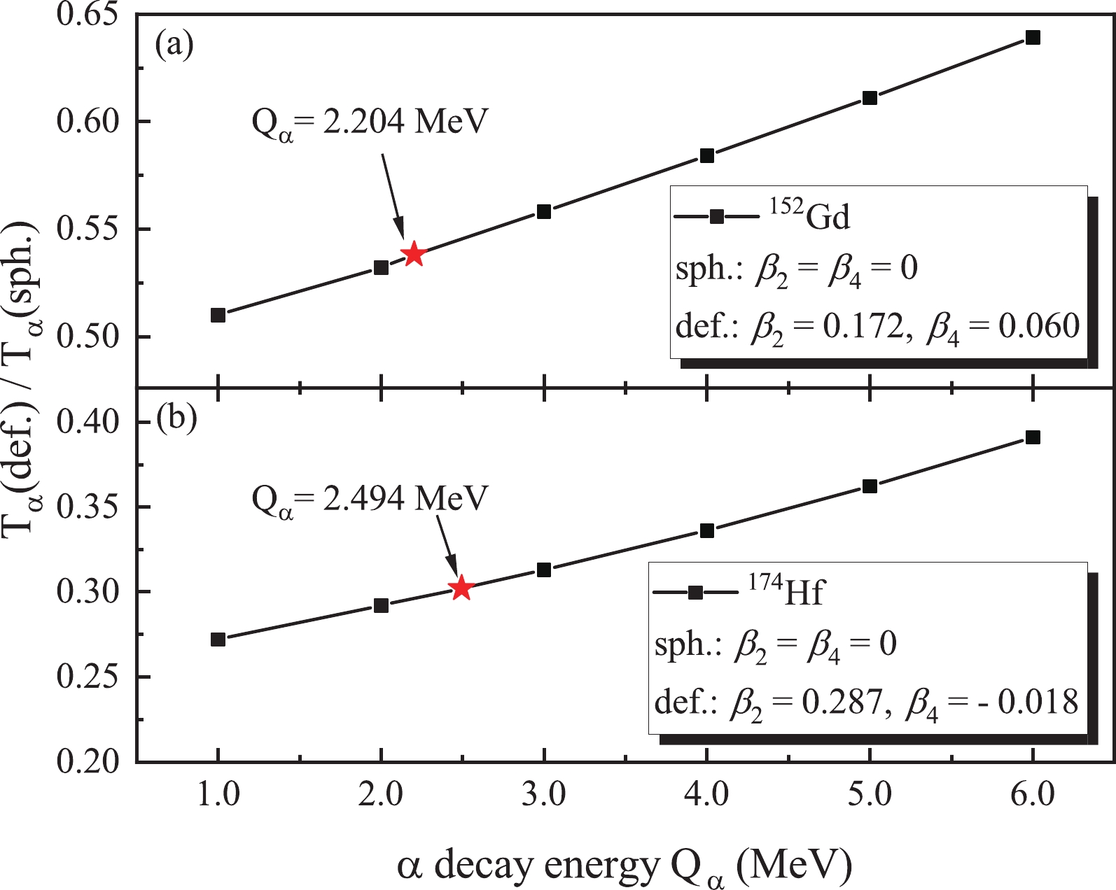

Figure 2.(color online) Ratios of theαdecay half-lives in the deformed case, $ T_\alpha $ (def.), to those in the spherical case, $ T_\alpha $ (cal.), as a function of theαdecay energy $ Q_\alpha $ for $ ^{152} $ Gd and $ ^{174} $ Hf. Experimental values are indicated by red stars.

Another factor that should be taken into account is the angular momentum carried by theαparticle. As shown inTable 1, six favoredαtransitions with $l=0$ are involved. The only exception is $^{209}$ Bi with a large angular momentum, $l=5$ . For this unfavoredαdecay, both the height and width of the Coulomb barrier are significantly increased by its centrifugal potential. The ratio of the corresponding decay width, Γ, with $l=5$ to $l=0$ for $^{209}$ Bi is $\dfrac{\Gamma_{l=5}}{\Gamma_{l=0}}\approx0.05$ . It should be interesting to discuss the correlation between theα-core potential and the corresponding bound state wave function of theαparticle for both favored and unfavored cases. The potentials and wave functions of $^{209}$ Bi $\rightarrow$ $^{205}$ Tl+αand $^{148}$ Sm $\rightarrow$ $^{144}$ Nd+αare plotted for better illustration. As shown inFig. 3(a), there exists a strong repulsive behavior of the potential, $U(r)$ , for $^{209}$ Bi in the inner part due to the angular momentum $l=5$ . Consequently, the corresponding bound state wave function, $\Phi_0(r)$ , of $^{209}$ Bi is pushed outwards compared with that of $^{148}$ Sm, as presented inFig. 3(b). Oscillations of the two wave functions are quite similar when $r , but the node numbers of $\Phi_0(r)$ for $^{209}$ Bi (blue line) and $^{148}$ Sm (red chain-dotted line) are $n=8$ and $n=9$ , respectively. The decay of $^{209}$ Bi involves a higher Coulomb barrier in the classically forbidden region. To be more specific, there is a difference of 3–4 MeV of $U(r)$ for $^{209}$ Bi and $^{148}$ Sm at $r=R_\text{sep}$ . As a result, one can see from the right panel ofFig. 3(b) that the bound state wave functions for these two nuclei decrease exponentially in the outer region ( $r\geq R_\text{sep}$ ), and $\Phi_0(r)$ for $^{209}$ Bi decreases more quickly due to the differences between the Coulomb barriers of the two nuclei.

Figure 3.(color online)α-core potentials (a) and corresponding bound state wave functions (b) for $^{148}$ Sm $\rightarrow$ $^{144}$ Nd+αand $^{209}$ Bi $\rightarrow$ $^{205}$ Tl+α, respectively. The separation point, $r=R_\text{sep}$ , is indicated both in (a) and (b). $r_1$ and $r_2$ in (a) are the first and second classical turning points, respectively.

For the twenty selected long-lived nuclei, the predictedαdecay half-lives, $ T_\alpha $ , calculated using the latest nuclear mass data [46] are listed inTable 2. The second, third, and fourth columns inTable 2present the current half-life limit, isotopic abundance (IS), and possible decay modes for each nucleus [46]. Listed in the fifth column are theαdecay energies taken from Ref. [46]. One can find that theαdecay energies of the nuclei are in the range of 1.0 MeV $ < Q_\alpha < 2.8$ MeV. Among them, $ ^{187} $ Os is found to have the largestαdecay energy with $ Q_\alpha = 2.722 $ MeV. It is well-known that the decay width is closely dependent on the decay energy, and the larger the decay energy, the easier the penetration of the preformedαcluster through the Coulomb barrier. The sixth and seventh columns present the deformation parameters of the daughter nuclei. As shown inTable 2, all nuclides except $ ^{142} $ Ce investigated here decay to a deformed nucleus since they are located in the open-shell region between the magic neutron numbers $ N = 82 $ and $ N = 126 $ . In particular, the nuclei with mass numbers ranging from $ A = 160 $ to $ A = 190 $ are largely deformed ( $ ^{162} $ Er $ - $ $ ^{190} $ Os). Similarly, the deformation effects are taken into account in the calculation through the averaging procedure. A $ 100\% ~~ g.s. $ to $ g.s. $ transition is assumed since the values of branching ratio, $ b_{\alpha}$ %, are unknown. The predictedαdecay half-lives are then given, which vary by several orders of magnitude from $ 10^{16} $ y to $ 10^{66} $ y. The fastest one among these possibleαemitters is $ ^{187} $ Os, for which the predictedαdecay half-life is $ T_\alpha $ = 4.57 $ \times10^{16} $ y. However, the isotopic abundance of $ ^{187} $ Os is rather low (IS = 1.96%), which adds another layer of difficulty in observing theαdecay events. As compared with $ ^{187} $ Os, $ ^{149} $ Sm is more abundant with IS = 13.82%, for which the predictedαdecay half-live is $ T_\alpha $ = 4.80 $ \times10^{18} $ y. For other nuclides, the predictedαdecay half-lives are many orders of magnitude longer than the theoretical $ T_\alpha $ of $ ^{187} $ Os and $ ^{149} $ Sm. It can be quite difficult to observe theirαdecays with the present experimental sensitivities. Thus, $ ^{187} $ Os and $ ^{149} $ Sm are recommended for future experiments searching for new long-livedαemitters.

Finally, it is worth noting that the calculation of theαdecay width for deformed nuclei within the averaging procedure is an approximate treatment. Several other approaches forαdecay of deformed nuclei can be applied, such as the coupled channel approach or theα-plus-rotor model. In general, theαdecaying state of deformed nuclei should be described by a three-dimensional quasi-stationary state wave function. A multidimensional approach should be developed for the tunneling of theαparticle through a deformed Coulomb barrier. For instance, one can solve a three-dimensional Schrödinger equation to obtain the decay width, Γ, by a number of methods: (i) grid-based approach [54], (ii) imaginary time propagation method [55] (iii), basis expansion method [56],etc. However, the solution of the three-dimensional Schrödinger equation is quite complex and limited by the matrix size or the number of bases. For wave functions at large separation, $ r = R_\text{sep} $ , the computation procedure could be rather time-consuming. The calculation providing a solution to the three dimensionalαdecay is undergoing.

Theαdecay half-lives of naturally occurring nuclei with extremely long half-lives are investigated with the latest experimental data. By using the two potential approach, the narrowαdecay width is expressed as a product of the bound state and scattering state wave functions of theαparticle. The half-lives ofαemitters are significantly decreased due to the deformations of the daughter nuclei, especially for low decay energy, $ Q_\alpha $ . For available long-livedαemitters with rather low decay energies, the agreement between the theoreticalαdecay half-lives and the experimental data is reasonable. Moreover, theαdecay half-lives of twenty candidates with low decay energies are predicted, for whichαdecays are energetically allowed but have not yet been observed. In particular, $ ^{187} $ Os is found to have the shortestαdecay half-life with $ T_\alpha = 4.57\times10^{16} $ y, followed by $ ^{149} $ Sm with $ T_\alpha = 4.80\times10^{18} $ y. It is considered that the observations ofαdecays for both $ ^{187} $ Os and $ ^{149} $ Sm are within the current experimental possibilities, which are strongly recommended for future experiments.