The entanglement properties of holographic QCD model with a critical end point

Entanglement plays a very important role in a strongly coupled system. In a quantum many body system, entanglement entropy is a measurement of quantum correlation between different parts of the system [1]. In the case of AdS/CFT correspondence or more general Gauge/Gravity duality [2-5], the holographic entanglement entropy provides insights into quantum information and quantum gravity [6-10].

From quantum field theory, e.g., quantum chromodynamics (QCD), the entire system is represented in 4-dimensional Minkowski spacetime, and for any state at a fixed time $ t_0 $ , we have the state vector $ |\Psi(t_0) \rangle $ and the density matrix given as

To investigate the entanglement entropy between different parts of this system, we first divide the entire time slice into two parts, which we denote asAand $ \bar{A} $ , whereAis a subregion of the time slice and $ \bar{A} $ is its complement. We then obtain the reduced density matrix of the subsystemAby tracing out the degree of freedom of subsystem $ \bar{A} $ in the Hilbert space

The entanglement entropy of subsystemAcan be defined as the von Neumann entropy [1]

However, it is not easy to directly calculate the entanglement entropy in the QCD side using this formula. According to the AdS/CFT correspondence or AdS/QCD correspondence [5,11-14] we know that the holographic duality of the entanglement entropy between boundary regionAand its complement is the holographic entanglement entropy which can be calculated using the Ryu-Takayanagi formula [15,16] as follows:

where $ m(A) $ is a 3-dimensional surface in the bulk which is homologous toA. The holographic entanglement entropy is equal to the minimal area $ m(A) $ , which is denoted as $ \gamma_A $ (the R-T surface) divided by a constant $ 4G_N $ . There have been several studies on the relationship between the holographic entanglement properties and the phase transition in holographic QCD models [17-22]. In a previously published report [17], the behavior of holographic entanglement entropy with temperature at the zero baryon chemical potential was investigated. In a separate study [18], the authors investigated holographic entanglement entropy in a strip shaped region in a holographic QCD model. Both studies determined that holographic entanglement entropy is sensitive to the phase transition of QCD matter.

Another very important aspect of holographic entanglement entropy is the shape dependence of the subregionA[23-25]. Since QCD theory applies to 4-dimensional spacetime, it is very difficult to calculate the holographic entanglement entropy for a general shaped regionA. Therefore, we consider two different shapes in our work to study the shape dependence of regionA. One is a spherical shaped region and the other is a strip shaped region.

For a thermal system with finite temperatureTand chemical potential $ \mu $ , entanglement entropy is not a reliable parameter for the measurement of the entanglement between different subsystems because of the thermodynamic contributions. To further elaborate on this concept, let us consider the purification of the quantum state on the boundary of a Schwarzschild-AdS black hole. It has been shown that the purified state lives on the double boundary of the bulk spacetime, which can be denoted asBand $ \bar{B} $ . If we divideBinto two disjointed subregionsAand $ \bar{A} $ , the holographic entanglement entropy of subregionAmeasures the entanglement betweenAand its complement $ \bar{A}\cup \bar{B} $ (but not $ \bar{A} $ ) [26]. By using the subadditivity and strong subadditivity of entanglement entropy, one can define two nonnegative entanglement quantities, the mutual information $ MI(A,B) $ and conditional mutual information $ CMI(A,B|C) $ , as [15,16]

It is believed that mutual information and conditional mutual information are better quantities for the measurement of the entanglement between different subsystems of a thermal system, compared to the entanglement entropy. However, these two quantities are simply the linear combination of entanglement entropy and not new quantities that describe entanglement in a thermal state. In recent years, a new entanglement quantity based on the purification of the thermal state, called the entanglement of purification (Ep), has been investigated [27-31]. For a thermal state on the boundary time slice, two unintersected subsystemsAandBchosen on the thermal state $ \rho_{AB} $ can be purified as

where $ |\sqrt{\rho}\rangle\langle\sqrt{\rho}| = \rho $ is a pure state density matrix. Then, the entanglement of purification forAandBcan be defined as [32]

where $ \rho_{AA^{*} = Tr_{BB^{*}}(|\sqrt{\rho}\rangle\langle\sqrt{\rho}|)} $ , and $ S(\rho_{AA^{*}}) $ is the entanglement entropy associated with $ \rho_{AA^{*}} $ . It is difficult to determine the appropriate purification for a general $ \rho_{AB} $ for the field theory side. The holographic duality of Ep is believed to be the entanglement wedge cross section [27]

where $\Sigma^{\min}_{AB}$ is the minimal surface area in the entanglement wedge ofAandBthat ends on their R-T surface, as shown in Fig. 12. The blue regions are the subregionsAandB, and the red surfaces are the R-T surfaces of $ A\cup B $ . The green surface is the minimal surface $\Sigma^{\min}_{AB}$ .

The remainder of this report is arranged as follows. In section II, we describe the model setting used in this work. In section III, we initially analytically compute the holographic entanglement entropy and derive the minimal area equations. We then analyze the numerical results for holographic entanglement entropy and compare it to the black hole entropy. We also investigate the behavior of other entanglement quantities such as mutual information, conditional mutual information, and entanglement of purification on the phase diagram in section IV. Finally, the conclusion and discussion are presented in section V.

The holographic QCD model we consider in this work is a 5-dimensional Einstein-Maxwell-dilaton holographic model, which is described as follows [33]:

where $ \kappa^2 $ is the gravitational constant, and $ \kappa^2 = 8\pi G_N $ ;gis the determinant of the 5-dimensional metric $ g_{\alpha\beta} $ . The first termRis the Ricci scalar, which corresponds to the QCD vacuum sector. The scalar field, $ \phi $ , corresponds to the gluon scalar condensate, and $ F_{\mu\nu}: = \partial_{\mu}A_{\nu}-\partial_{\nu}A_{\mu} $ is the strength tensor of a $ U(1) $ gauge field $ A_{\mu} $ , which gives the quark chemical potential and density. We then take the ansatz of the asymptotic AdS $ _5 $ metric as follows [33]:

wherezis the holographic direction of the asymptoticAdS $ _5 $ , and $ z = 0 $ corresponds to the ultra-violet (UV) boundary spacetime for which the QCD theory is applicable. Following [33], the dilaton field and the gauge field take the forms of

Using the regular boundary conditions at the horizon $ z = z_H $ and the asymptotic $ AdS_5 $ conditions at the UV boundary $ z = 0 $ [33], we have

where $ \mu $ and $ \rho $ are the baryon chemical potential and density, respectively. The warped factor and gauge kinetic function can be fixed as [33]

By solving the equation of motion we get [33]

We can also calculate the baryon density $ \rho $ and the temperatureTas [33]

Then, by fitting the vacuum vector meson mass $ m_{\rho} = $ 0.77 GeV and the phase transition temperature $ T_c = $ 0.17 GeV at $ \mu = 0 $ , we can fixcandbas in [33]:

Based on the preceding parameters, the phase diagram for deconfined phase transition of the holographic QCD model of [33] is shown inFig. 1.

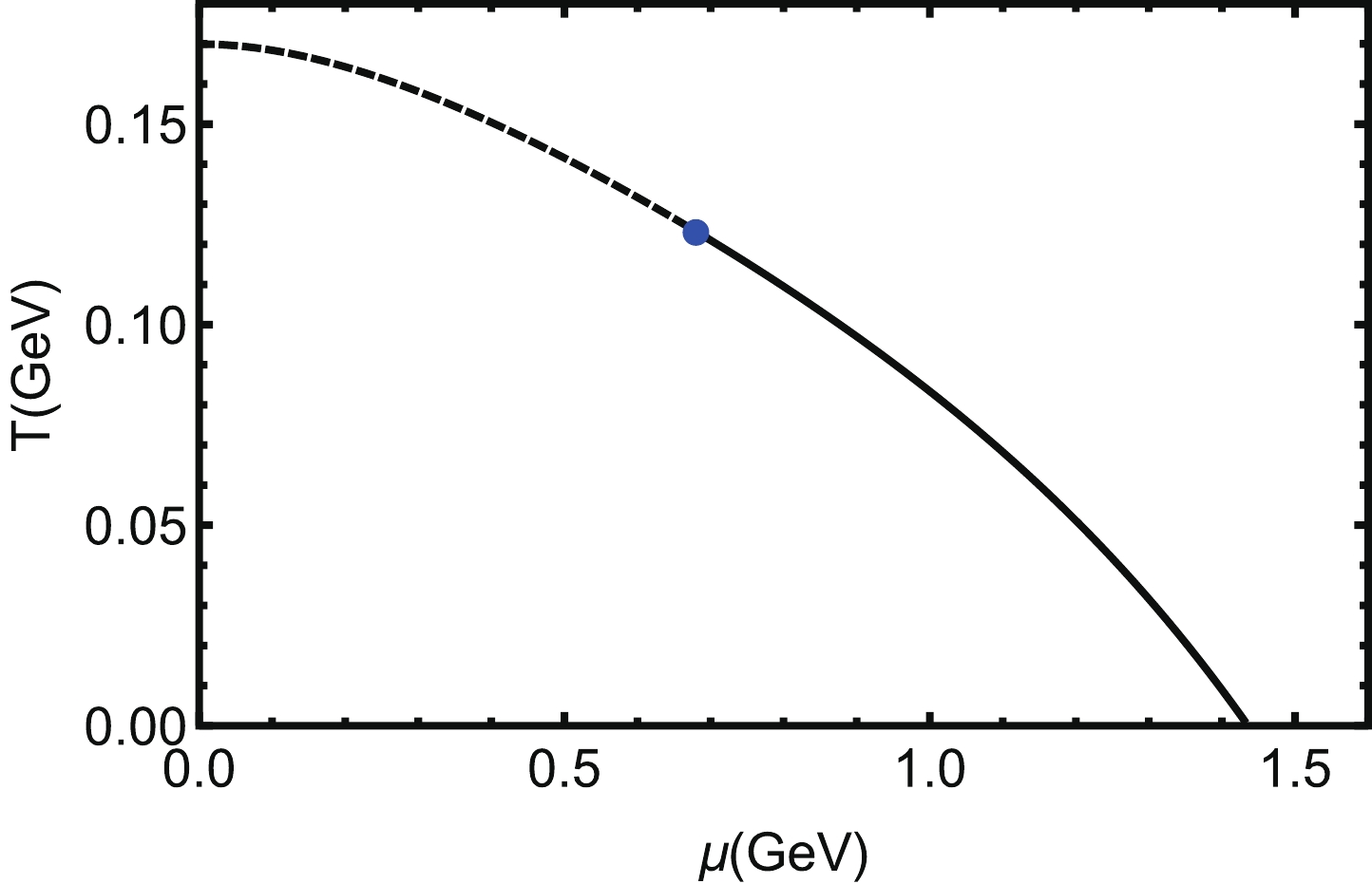
Figure 1.The phase diagram of the holographic QCD model used in this work [33]. The dashed line is the phase boundary of the crossover region ( $\mu < 0.693 \;{\rm{GeV}}$ ), the blue dot is the CEP located at ( $\mu^E = 0.693 \;{\rm{GeV}}$ , $T^E = 0.121 \;{\rm{GeV}}$ ), and the solid line is the first order phase boundary ( $\mu > 0.693 \;{\rm{GeV}}$ ).

The dashed line is the phase boundary of the crossover region ( $ \mu < 0.693 \;{\rm{GeV}} $ ), the blue dot is the CEP located at ( $ \mu^E = 0.693 \;{\rm{GeV}} $ , $ T^E = 0.121 \;{\rm{GeV}} $ ), and the solid line is the first order phase boundary ( $ \mu > 0.693 \;{\rm{GeV}} $ ). The black hole entropy of this system can be derived as:

It is evident that this black hole entropy is divergent. However, given that we need to determine the relationship between the temperature,T, and baryon chemical potential, $ \mu $ , of the black hole entropy, we can exclude the divergent part and define the entropy density as follows:

In this section, we will consider the holographic entanglement entropy in the holographic QCD model that was defined in the last section. In this work, we choose the subregionAto be highly symmetric: 1) a spherically-shaped region on the boundary time slice with $ 0\leqslant \vec{x}^2\leqslant r^2_0 $ is shown inFig. 2; 2) a strip-shaped region on the boundary time slice with $ -a/2\leqslant x_1\leqslant a/2 $ and $ -\infty for $ i = 2,3 $ is shown inFig. 3. The blue region is regionA, and the red region is the surface, $ \gamma_A $ ,which is the minimal surface that is homologous toAin the bulk. It will be very convenient to transform to spherical coordinates for the spherical shaped regionA,for which this region will be $ 0 , as represented by the blue line inFig. 2, and the red line is the minimal surface, $ \gamma_A $ .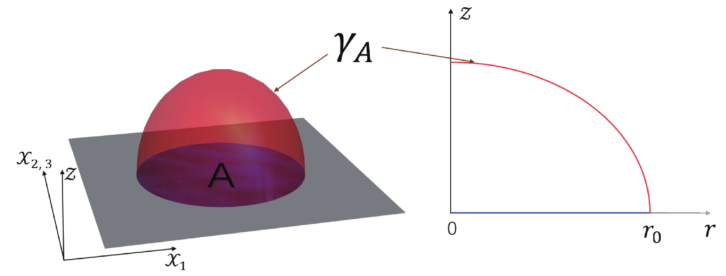

Figure 2.(color online) (Left) The spherical shaped subregionA(the blue region) and the minimal surface, $\gamma_A$ , (the red surface). (Right) In spherical coordinates, we only need to consider the direction of the radius. RegionAis from $r = 0$ to $r = r_0$ and the minimal surface, $\gamma_A$ , can be determined by $z = z(r)$ , which is the solution of the minimal area equation.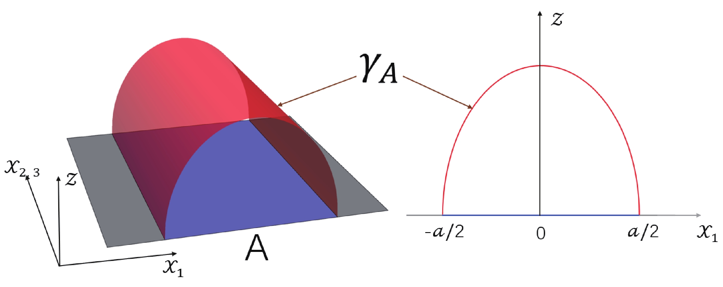

Figure 3.(color online) (Left) The strip shaped subregionA(the blue region) and the minimal surface, $\gamma_A$ , (the red surface). (Right) Given the symmetry of regionA,we only need to consider the $x_1$ direction, and this region is defined by $-a/2 (the blue line) . The minimal surface, $\gamma_A$ , is determined by $z = z(x_1)$ , which is the solution of the minimal area equation.

For a spherical shaped regionAshown inFig. 2, the area of $ m(A) $ with $ m(A): z = z(x_1, x_2, x_3) $ is given by

wherehis the determinant of the reduced metric on surface $ m(A) $ . After transforming to spherical coordinates, we have $ z = z(r, \theta, \phi) $ . We then exploit the symmetry of regionAand the bulk time slice since the minimal surface should have the same symmetry withA.This means that we only need to consider surfaces defined by $ z = z(r) $ as shown inFig. 2. Thus, we have

The minimal area equation can be calculated as

with the boundary conditions

we can solve the minimal area equation with the solution $ z = z_m(r) $ . Then, the area of the minimal surface is given by

and the holographic entanglement entropy for a spherical shaped region is given as

For a strip shaped regionA,as shown inFig. 3, the area of surface $ m(A) $ is

It should be noted that, in this case, we denote the determinant of the reduced metric on surface $ m(A) $ byh. Moreover, using the symmetry of regionAand the bulk time slice, it can be determined that the minimal surface should have the same symmetry withAand can be defined by $ z = z(x_1) $ as shown inFig. 3. We then obtain the area of $ m(A) $

where $ M_1 $ and $ M_2 $ are the lengths of regionAalong the $ x_2 $ and $ x_3 $ directions, respectively. The minimal area equation can then be expressed as

We can then solve this minimal area equation using the following boundary conditions:

or equally

Pluging the solution of the minimal area equation $ z = z_m(x_1) $ into the area formula, we obtain the area of the minimal surface $ \gamma_A $

The holographic entanglement entropy for a strip shaped region is given as

In this section, we first provide the numerical results for the black hole entropy of the holographic QCD model; then, we show the numerical results for the holographic entanglement entropy of a spherical shaped region and a strip shaped region.

Before we show the entanglement entropy on the QCD phase diagram, we first calculate the black hole entropy for different temperatures,T, and the baryon chemical potential, $ \mu $ . We initially fix the constant $ \kappa^2 = 1 $ in the following calculation. In this case, we choose the divergent term to be

and note that we can fix this term to be any constant in principle. Then, the black hole entropy $ S_{bh} $ for a fixed $ \mu $ as a function of the temperature is shown inFig. 4.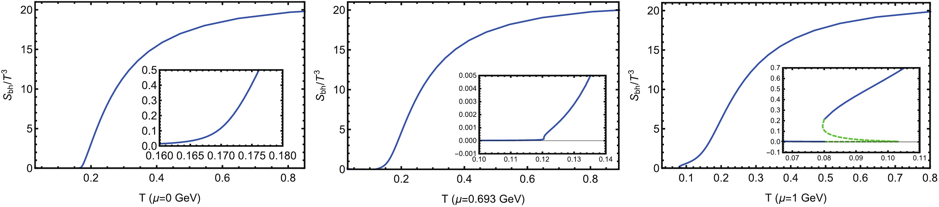

Figure 4.(color online) The scaled black hole entropy $S_{bh}/T^3$ as a function of temperature for different quark chemical potentials. The blue solid lines are the physical black hole entropy from the minimal of the free energy. At $\mu = 0$ , phase transition occurs at $T = 0.17\; {\rm GeV}$ , and it is a crossover, so $S_{bh}$ is single valued and smooth. When $\mu = 0.693\; {\rm{GeV}}$ , it is the critical endpoint of the first order phase transition and the transition temperature is $T = 0.121\; {\rm{GeV}}$ , where $S_{bh}$ is single valued but not smooth. For $\mu = 1\; {\rm{GeV}}$ , the first order phase transition occurs at $T = 0.08\; {\rm{GeV}}$ for which $S_{bh}$ is not single valued, and the physical value of $S_{bh}$ is not continuous at this point.

The blue solid line is the physical value of $ S_{bh}/T^3 $ . For the first order phase transition, the green dashed line does not physically correspond to the metastable state determined by the maximum of the free energy [33]. It is observed that at different chemical potentials, the black hole entropy, $ S_{bh} $ , or equally, $ S_{bh}/T^3 $ , is almost zero in the hadron phase and then sharply increases at the phase boundary. At a very high temperature, the ratio of $ S_{bh}/T^3 $ has a constant value of approximately $ 20 $ for all temperatures. We then focus on the behavior of the black hole entropy at the phase boundary. It is determined that in the crossover region ( $ 0\leqslant \mu < 0.693 $ $ {\rm{GeV}} $ ), the ratio of $ S_{bh}/T^3 $ is single valued and smooth. At the CEP ( $ \mu^E = 0.693\; {\rm{GeV}} $ , $ T^E = 0.121\; {\rm{GeV}} $ ), the ratio of $ S_{bh}/T^3 $ is single valued but not smooth. Moreover, in the first order phase transition region ( $ 0.693\; {\rm{GeV}} <\mu $ ), the ratio of $ S_{bh}/T^3 $ is not single valued, which means that the ratio of $ S_{bh}/T^3 $ is not continuous at the first order phase boundary. As such, the black hole entropy or the normalized black hole entropy is simply the holographic duality of the entropy of thermal QCD.

In what follows, we will perform numerical calculation of the holographic entanglement entropy for a spherical shaped region and a strip shaped region. It should be noted that to obtain a finite area of the minimal surface, we also need to choose a UV-cutoff because of the boundary UV-divergence at $ z = 0 \; {\rm{GeV}}^{-1} $ , which is called the renormalization of the holographic entanglement entropy [15,16].

Firstly, we take the UV-cutoff to be $ z = \epsilon $ , and the area of minimal surface for a spherical shaped region and the strip shaped region are given as

We choose $ \epsilon = 0.01\; {\rm{GeV}}^{-1} $ in our calculation, and therefore, $ \epsilon_0 $ is not a constant but a function of temperatureTand the quark chemical potential $ \mu $ , e.g., $ \epsilon_0 = \epsilon_0(T, \mu) $ as shown inFig. 5.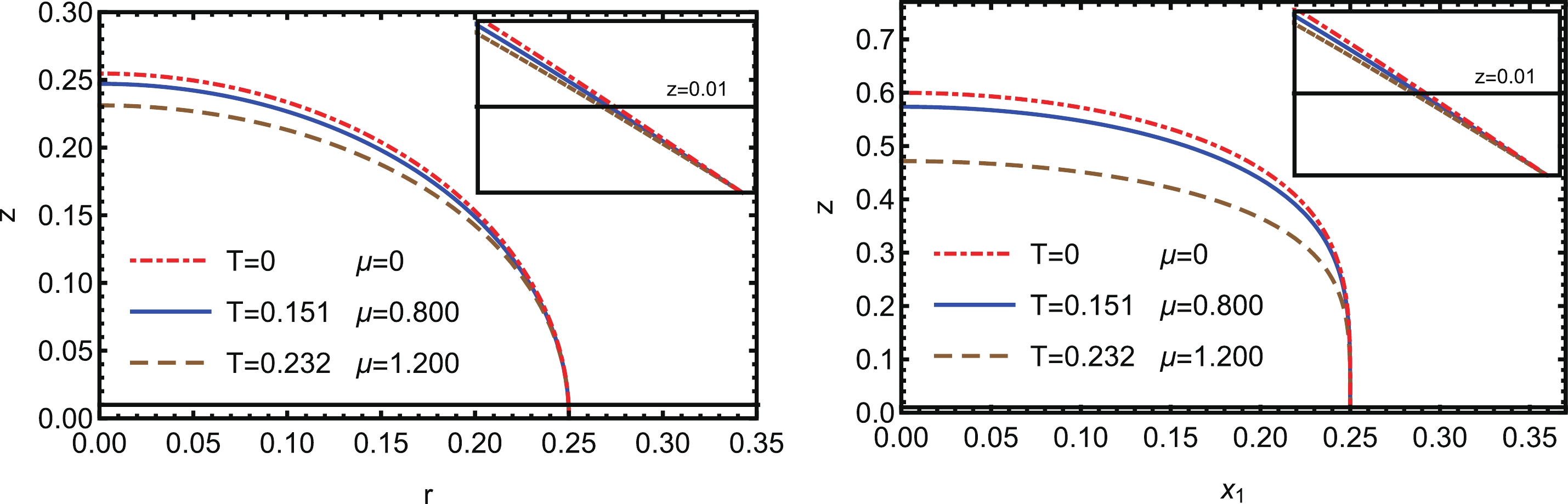

Figure 5.(color online) The minimal surface with a UV-cutoff at $z = 0.01$ ${\rm{GeV}}^{-1}$ for different temperatures and baryon chemical potentials. (Left) The minimal surface for a spherical shaped regionA. (Right) The minimal surface for a strip shaped regionA. In this case, the unit for the temperature and the chemical potential $\mu$ is ${\rm{GeV}}$ .

Every minimal surface for differentTand $ \mu $ ends at the same point on the boundary with $ z = 0 $ $ {\rm{GeV}}^{-1} $ . After taking the UV-cutoff, different surfaces have different boundaries on the slice of $ z = 0.01 \; {\rm{GeV}}^{-1} $ . For the strip shaped regionA, we also need to consider the parameters $ M_1 $ and $ M_2 $ to be finite, and we choose $ M_1 = M_2 = 1 $ and $ r_0 = a/2 = 0.25\; {\rm{GeV}}^{-1} $ . Then, within the holographic QCD model and using the holographic entanglement entropy formulae Eqs. (38) and (39), we can calculate the holographic entanglement entropy between the two subregionsAand $ \bar{A} $ for different temperaturesTand baryon chemical potentials $ \mu $ .Fig. 6shows the 3D-plot of the holographic entanglement entropy on the $ (T,\mu) $ plane and the 2D-plot along the fixed baryon chemical potential line. It should be noted that the physical entanglement entropy could be determined from the minimal value of the free energy.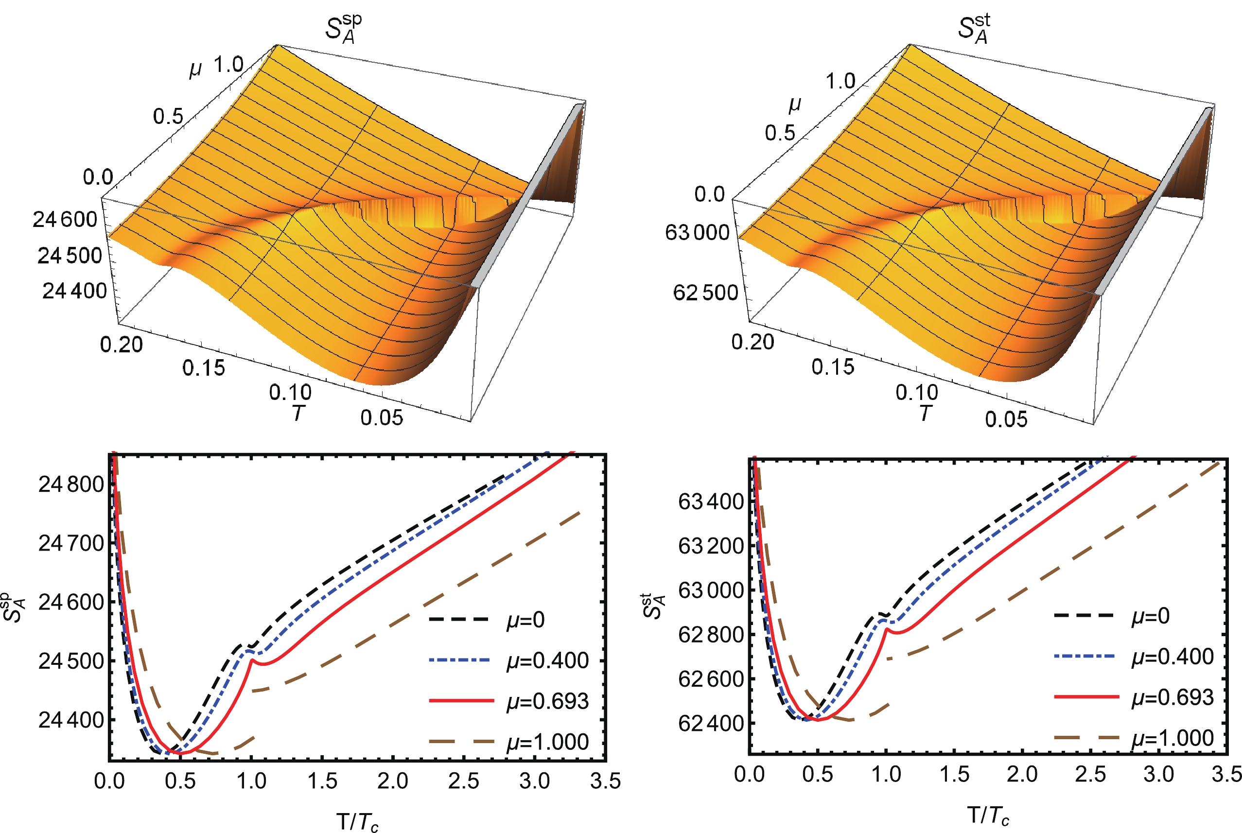

Figure 6.(color online) 3D-plot of the holographic entanglement entropy on the $(T,\mu)$ plane and the 2D-plot along the fixed baryon chemical potential line. The unit for the temperatureTand the chemical potential $\mu$ is ${\rm{GeV}}$ .

FromFig. 6, it is evident that the holographic entanglement entropies of a spherical shaped region, $ S_A^{sp} $ , and the strip shaped region, $ S_A^{st} $ , are very similar on the $ (T,\mu) $ phase diagram. In the crossover region, both $ S_A^{sp} $ and $ S_A^{st} $ decrease initially at a low temperature, then increase, and then decrease again. Thus, a weak peak structure is formed around the phase boundary, which then increases sequentially in the QGP phase. However, it should be noted that although $ S_A^{sp} $ and $ S_A^{st} $ have very similar increasing and decreasing behavior on the phase diagram, they have different values for fixedTand $ \mu $ . Near the phase boundary, $ S_A^{sp} $ and $ S_A^{st} $ change smoothly in the crossover region and form a weak peak structure in the vicinity of the phase boundary. However, we find that the top of the peak is not exactly the phase boundary. At CEP ( $ \mu^E = 0.693 $ $ {\rm{GeV}} $ $ T^E = 0.121 $ $ {\rm{GeV}} $ ), $ S_A^{sp} $ and $ S_A^{st} $ are continuous but not smooth. In addition, it should be noted that the CEP is exactly at the top of the peak in the vicinity of the phase boundary. In the first order phase transition region, $ S_A^{sp} $ and $ S_A^{st} $ are not continuous at the phase boundary. These continuity properties are very similar to the case of the black hole entropy $ S_{bh} $ , and therefore, the holographic entanglement entropy of different boundary regions could also be a signal of QCD phase transition. However, it should be noted that several investigations [17,18] have revealed a model dependence on the behavior of entanglement entropy in the phase diagram. Therefore, it is difficult provide a robust theoretical interpretation of this behavior of the entanglement entropy. However, despite the model dependence, it is evident that the behavior of entanglement entropy in the phase diagram is sensitive to the phase transition of quark matter.

In section III B.1, we concluded that the black hole entropy is the holographic duality of the thermal entropy of the QCD. Lattice results [34] show that the thermal entropy $ S_{th} $ has the behavior $ S_{th}\sim T^3 $ at high temperatures with $ \mu = 0 $ . It is evident that the black hole entropy, $ S_{bh} $ , has the same property but the holographic entanglement entropy does not. At high temperatures, the behavior of holographic entanglement entropy is most likely to be proportional toTwith $ \mu = 0 $ as shown inFig. 7.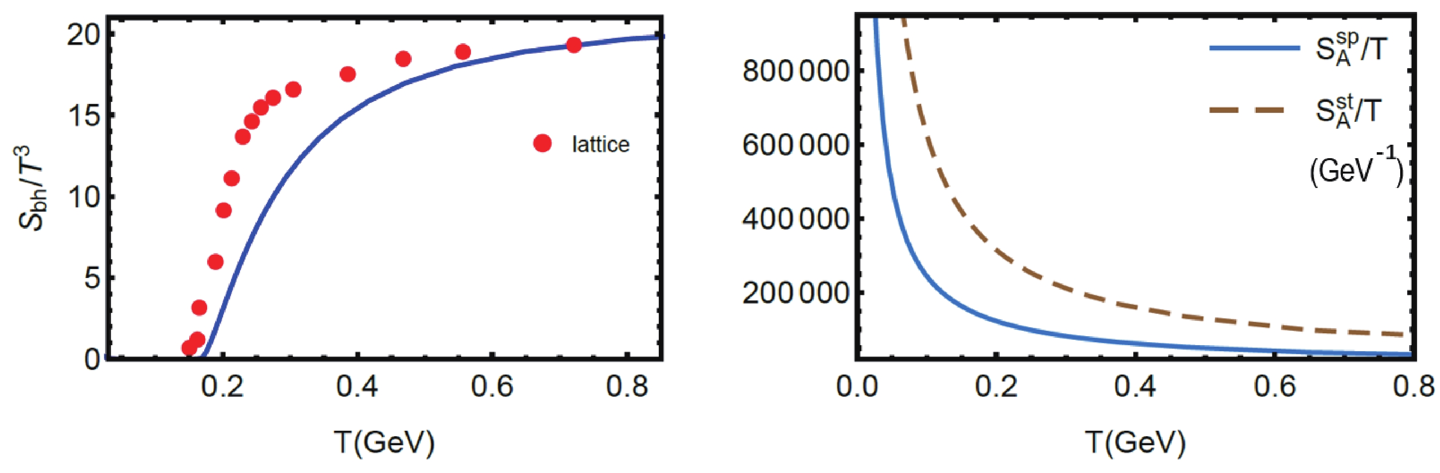

Figure 7.(color online) The behavior of black hole entropy and entanglement entropy at high temperatures with $\mu = 0$ . (Left) The red dots are the lattice data [34] of thermal entropy, and the blue solid line is the black hole entropy in our holographic QCD model. (Right) $S_A^{sp}/T$ and $S_A^{st}/T$ at $\mu = 0$ .

The black hole entropy, $ S_{bh}/T^3 $ , represented as the solid line in the left figure matches the lattice result for the thermal entropy, $ S_{th}/T^3 $ , and they both assume constant values. The holographic entanglement entropy for both regions is proportional toTat high temperatures when $ \mu = 0 $ .

The entanglement entropy measures the strength of the entanglement between different subsystems when the entire system is in a pure state. However, for a thermal state system, the entanglement entropy includes the contributions of the thermodynamics and not only the entanglement contributions. From the inequalities of entanglement entropy such as the subadditivity and the strong subadditivity, one can define other entanglement quantities. The two most often encountered quantities are called mutual information $ MI(A,B) $ (5) and conditional mutual information $ CMI(A,B|C) $ (6) [15,16]. Another useful entanglement quantity for the study of entanglement property in a thermal system is the entanglement of purification (8) and its holographic duality, the entanglement wedge cross section (9) [27,28].

In this section we only consider the strip shaped regionsAandBdefined as $ a\leqslant x_1\leqslant b $ and $ -\infty . If we fix their boundariesaandb, the regions will be defined. The three situations ofAandBthat are considered are shown inTable 1.

In this section, we consider the mutual information of two unintersected subsystemsAandBas shown inFig. 8.

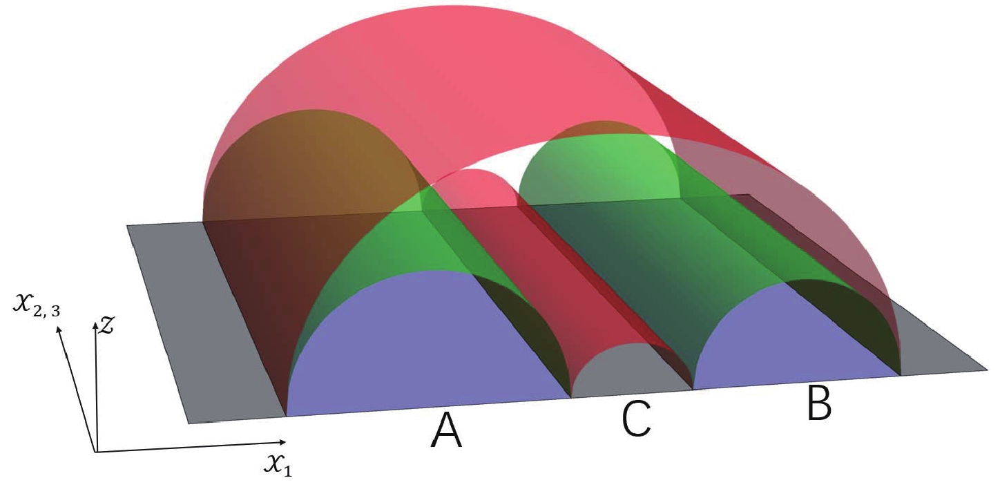
Figure 8.(color online) Mutual information. The green surfaces are the R-T surfaces ofAandB,and the red surfaces are the R-T surfaces of $ A\cup B$ .

Mutual information $ MI(A,B) $ is defined as follows:

We choose three nontrivial constructions ofAandBas shown inTable 1, such that $ MI(A,B)> 0 $ for any temperatureTand baryon chemical potential $ \mu $ . The holographic mutual information can then be calculated as

where ${\rm Area}(\Sigma_{\rm gre})$ ( ${\rm Area}(\Sigma_{\rm red})$ ) denotes the area of the green (red) surfaces as shown inFig. 8. It should be noted that the green surfaces are the R-T surfaces ofAandB, and the red surfaces correspond to the R-T surfaces of $ A\cup B $ . The numerical results of mutual information for different settings ofAandBare shown inFig. 9.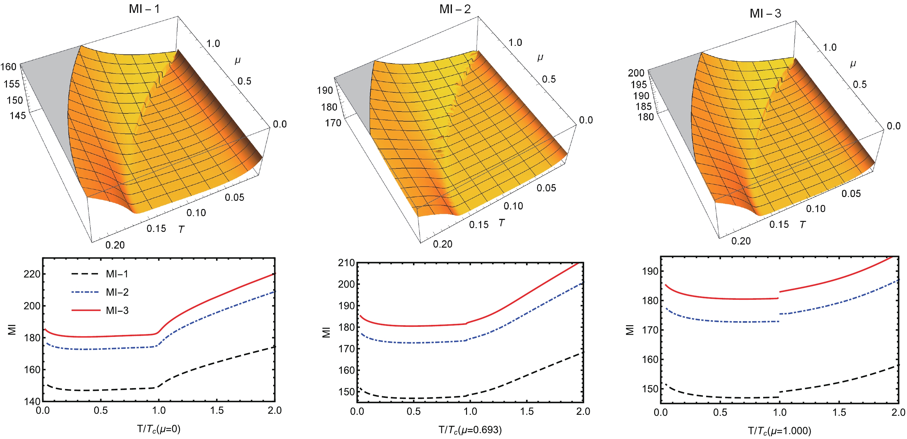

Figure 9.(color online) (Upper) 3D-plot of the mutual information on the $(T,\mu)$ plane and (Lower) the 2D-plot along the fixed baryon chemical potential line for cases 1, 2, and 3 ofAandBinTable 1. The unit for the temperatureTand the chemical potential $\mu$ is ${\rm{GeV}}$ .

We denote the mutual information $ MI(A,B) $ of the three cases ofAandBconsidered inTable 1as MI-1, MI-2 and MI-3 correspondingly. The upper sub-figure ofFig. 9shows the 3D-plot of the mutual information betweenAandBon the (T, $ \mu $ ) phase diagram. It is evident that $ MI(A,B) $ for different constructions ofAandBbehaves similarly on the phase diagram if we ignore its exact values but exhibits different behaviors for the entanglement entropy, as shown inFig. 6. $ MI(A,B) $ does not change significantly in the hadron matter phase but increases with the increase inTand $ \mu $ in the QGP phase. Similar to the entanglement entropy, in the crossover region, $ MI(A,B) $ is single valued and changes smoothly near the phase boundary. It is continuous but not smooth at the CEP and is not single valued (and so is not continuous) at the first order phase boundary. Not surprisingly, $ MI(A,B) $ is finite at anyTand $ \mu $ , although $ S(A) $ , $ S(B) $ , and $ S(AB) $ are divergent. The lower 2D-plot inFig. 9shows the same result. However, the 2D-plot gives another interesting result

Considering the symmetry of the bulk spacetime, we have ${\rm Area}(\Sigma_{\rm red}^1) = {\rm Area}(\Sigma_{\rm red}^2) = {\rm Area}(\Sigma_{\rm red}^3)$ . In this case, the superscripts represent the corresponding three cases ofAandB. Thus, this inequality implies that $ S(A)+S(B) $ decreases with the increase in $ |{\rm Area}(A)-{\rm Area}(B)| $ when $ {\rm Area}(A)+ $ ${\rm Area}(B) $ is a constant. $ {\rm Area}(A) $ and $ {\rm Area}(B) $ denote the area of subregionAandB, respectively. When $ {\rm Area}(A) = {\rm Area}(B) $ , $ S(A)+S(B) $ assumes the maximal value.

In this section, we consider the conditional mutual information of two unintersected subsystemsAandBas shown inFig. 10.

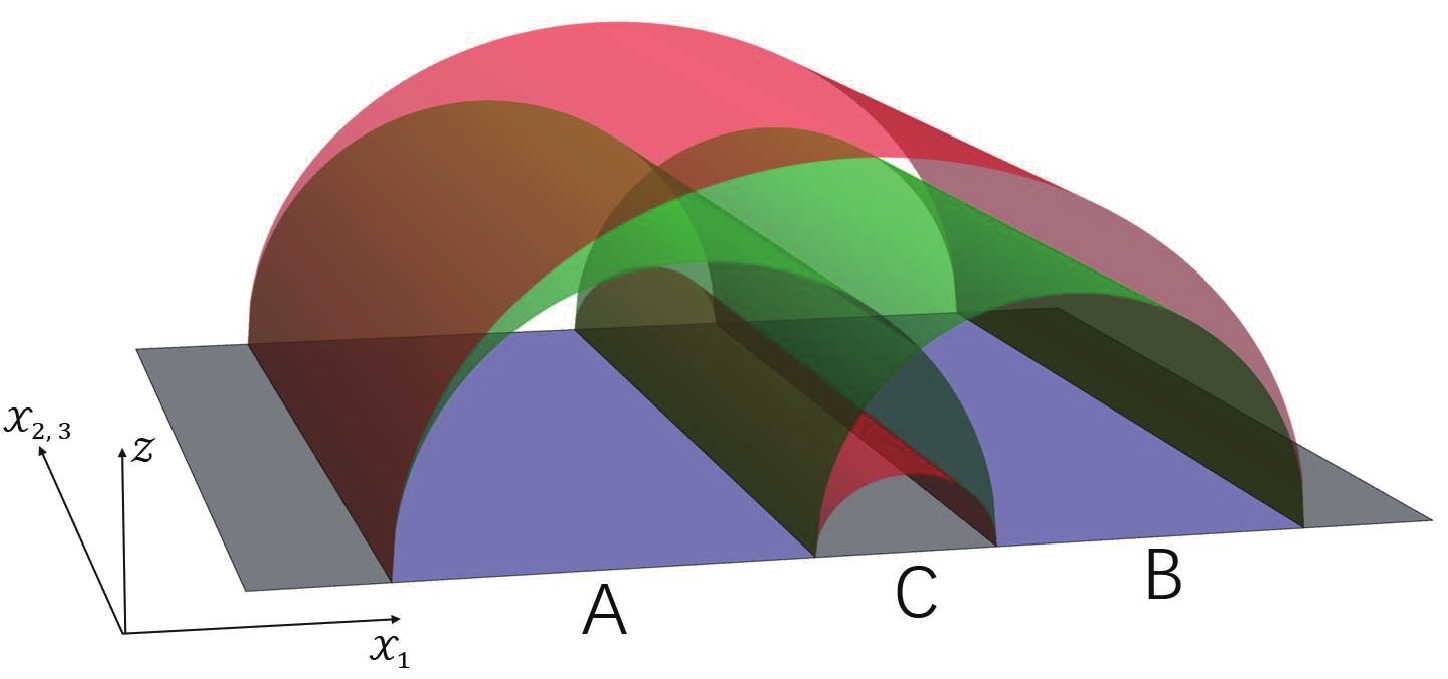
Figure 10.(color online) Conditional mutual information. The green surfaces are the R-T surfaces of $A\cup C$ and $B\cup C$ , and the red surfaces are the R-T surfaces ofCand $A\cup B\cup C$ .

The conditional mutual information is defined as

The holographic mutual information can then be calculated as

where ${\rm Area}(\Sigma_{\rm gre})$ ( ${\rm Area}(\Sigma_{\rm red})$ ) represents the area of the green (red) surfaces as shown inFig. 10. The green surfaces are the R-T surfaces of $ A\cup C $ and $ B\cup C $ , and the red surfaces correspond to the R-T surfaces of $ A\cup B\cup C $ andC.

For the conditional mutual information, we also consider the same regionsAandBas given inTable 1.Fig. 11shows the 3D-plot of $ CMI(A,B|C) $ on the (T, $ \mu $ ) phase diagram and its 2D-plot along a fixed $ \mu $ .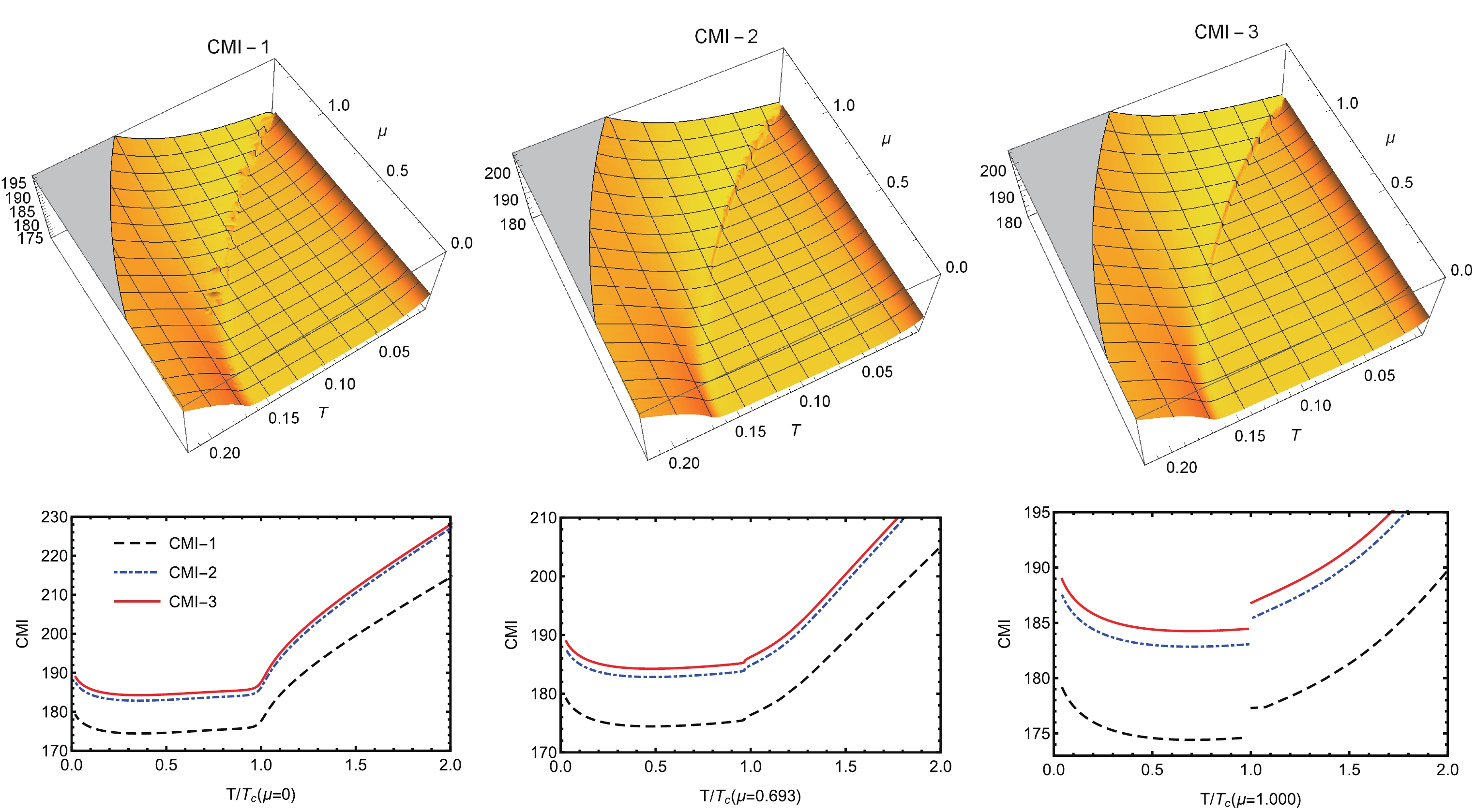

Figure 11.(color online) (Upper) 3D-plot of the conditional mutual information on the $(T,\mu)$ plane and (Lower) the 2D-plot along a fixed baryon chemical potential line for cases 1, 2, and 3 ofAandBinTable 1. The unit for temperatureTand the chemical potential $\mu$ is ${\rm{GeV}}$ .

It should be noted that similar to the case of mutual information, we also denote the three settings ofAandBas CMI-1, CMI-2, and CMI-3. For differentA,B, andC, $ CMI(A,B|C) $ also behaves similarly on the (T, $ \mu $ ) phase diagram but has different values. Moreover, the behavior of $ CMI(A,B|C) $ is very similar to that of $ MI(A,B) $ . It does not change significantly in the hadronic matter phase but increases rapidly with the increase inTand $ \mu $ in the QGP phase. Near the phase boundary, $ CMI(A,B|C) $ changes smoothly in the crossover region and continuously but not smoothly at CEP; it exhibits discontinuous behavior in the first phase transition region. This implies that $ CMI(A,B|C) $ could also be used to measure the entanglement between the subregionsAandB,and it describes the phase transition of strongly coupled matter. The lower 2D-plot inFig. 11exhibits the same results and also yields a similar inequality

Using the same argument in section IVA, firstly, considering the symmetry of the bulk spacetime, we have $ {\rm Area}(\Sigma_{\rm red}^1) = {\rm Area}(\Sigma_{\rm red}^2) = {\rm Area}(\Sigma_{\rm red}^3) $ . The superscripts represent the three cases ofAandB. Thus, the inequality implies that $ S(AC)+S(BC) $ decreases with the increase in $ |{\rm Area}(A\cup C)-{\rm Area}(B\cup C)| $ when $ {\rm Area}(A\cup C)+ {\rm Area} (B\cup C) $ is a constant; here, $ {\rm Area}(A\cup C) $ and $ {\rm Area}(B\cup C) $ correspond to the area of the subregions $ A\cup C $ and $ B\cup C $ , respectively. When $ {\rm Area}(A\cup C) = {\rm Area} (B\cup C) $ , $ S(AC)+ S(BC) $ assumes the maximal value.

In this section we consider the entanglement of purification of two unintersected subsystemsAandB, as shown inFig. 12. The holographic duality of entanglement of purification is the entanglement wedge cross section [27,28]

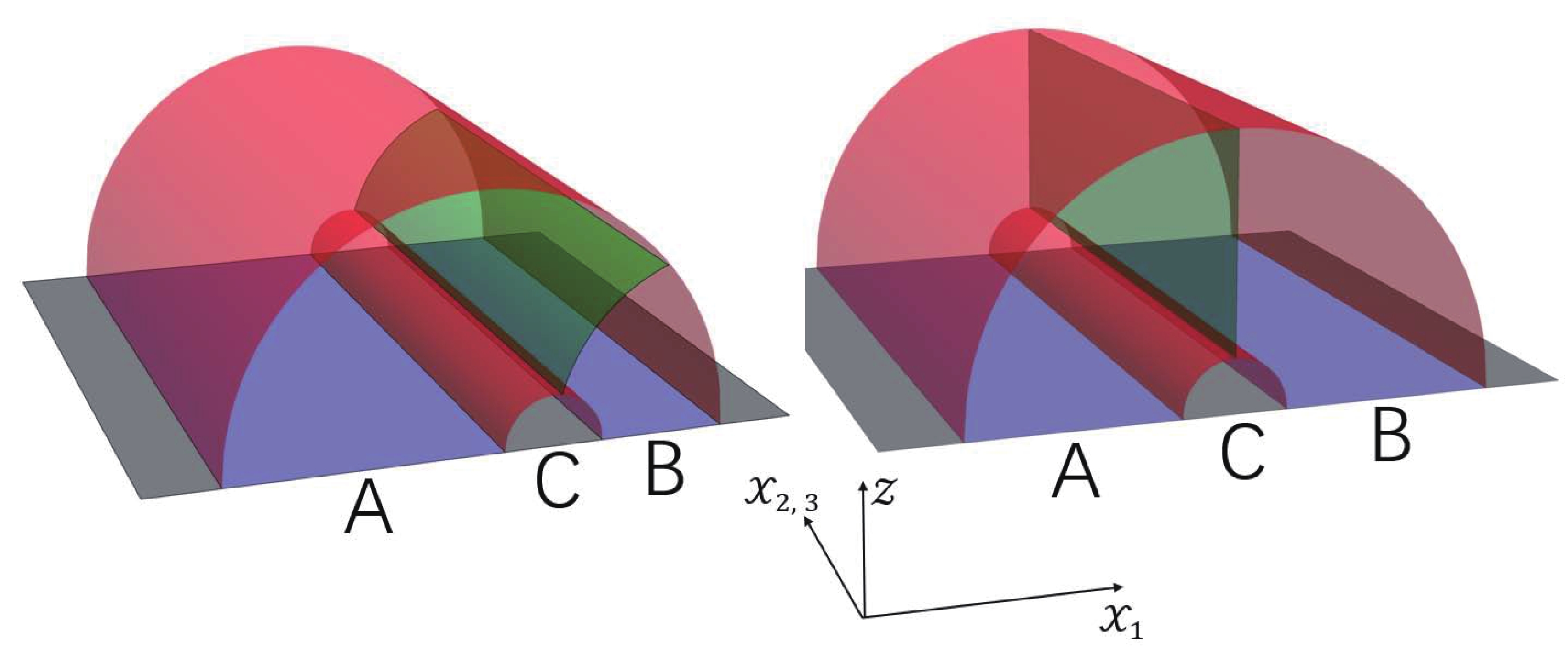
Figure 12.(color online) The entanglement of purification. (Left) The asymmetry case and (Right) the symmetry case ofAandB. The red surfaces are the R-T surfaces of $A\cup B$ , and the green surface gives the minimal cross section of the entanglement wedge ofAandB.

where ${\rm Area}(\Sigma_{\rm gre})$ represents the area of the green surfaces as shown inFig. 12.

In this section, we only consider the symmetric case ofAandB(case-3 inTable 1). The minimal surface is the surface with $ x_1 = const $ as shown in the right sub-figure inFig. 12. The asymmetric case ofAandBis potentially much more complicated, and we may consider it in our next work.Fig. 13shows the 3D-plot of $ Ep(A,B) $ on the (T, $ \mu $ ) phase diagram and its 2D-plot along a fixed $ \mu $ .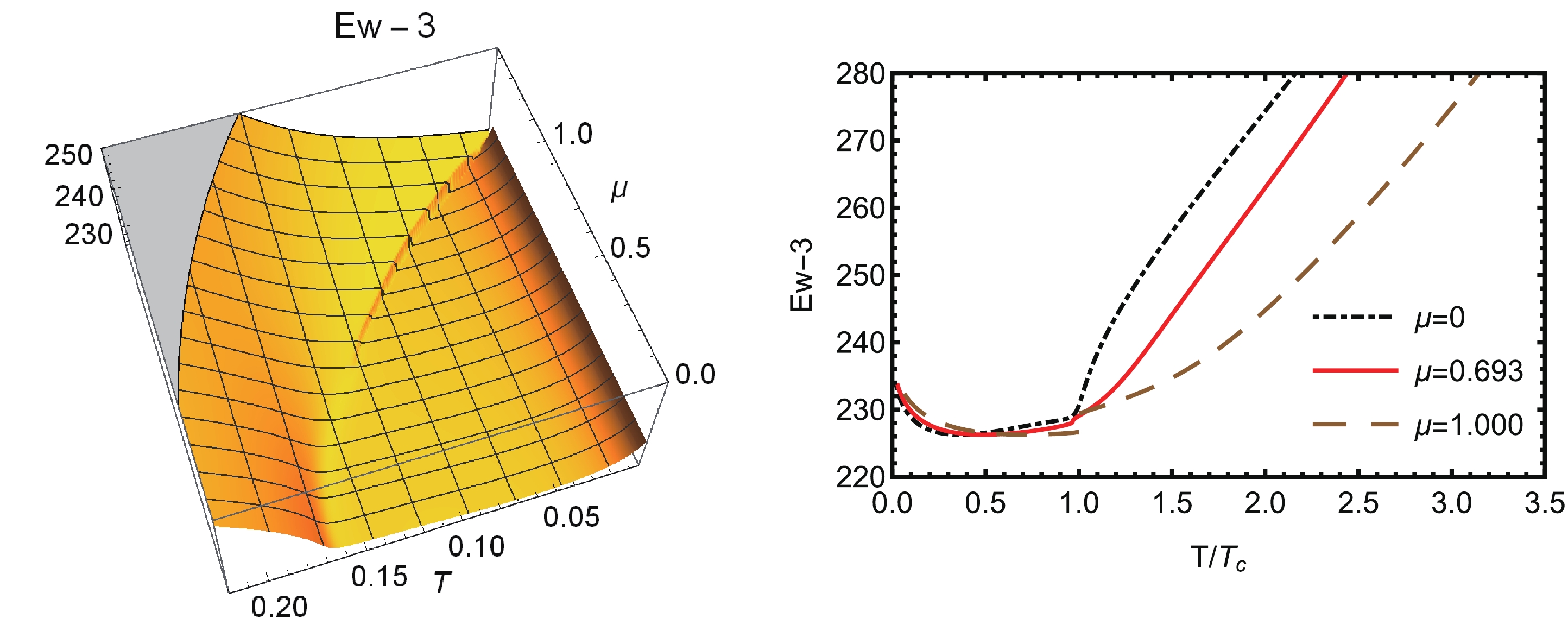

Figure 13.(color online) (Left) 3D-plot of the entanglement of purification on the $(T,\mu)$ plane and (Right) the 2D-plot along a fixed baryon chemical potential line for case-3 ofAandBinTable 1. The unit for the temperatureTand the chemical potential $\mu$ is ${\rm{GeV}}$ .

In [9], the authors propose that $ Ew(A,B) $ could be equal to the mutual information if a group of bit flow related to the mutual information is introduced, which can be limited within the entanglement wedge and ends onAandB. Moreover, in [27,28] the authors suggested that $ Ep(A,B) $ should be the holographic duality of the entanglement of purification ofAandB. The 3D-plot inFig. 13shows a very similar behavior of $ Ep(A,B) $ to $ MI(A,B) $ and $ CMI(A,B|C) $ , as shown inFig. 9andFig. 11. These similarities could also be observed inFig. 14, where we plot the $ MI(A,B) $ (red plot), $ CMI(A,B|C) $ (green plot), and $ Ep(A,B)-38 $ (blue plot). It should be noted that, to compare these three entanglement quantities, we only consider the symmetric case ofAandB(case-3 inTable 1). It is evident inFig. 14that for fixedTand $ \mu $ $ Ep(A,B)\geqslant CMI(A,B|C)\geqslant MI(A,B) $ . The second " $ \geqslant $ " is due to the monogamy of the mutual information. If we consider the mutual information ofA,B,andC,we have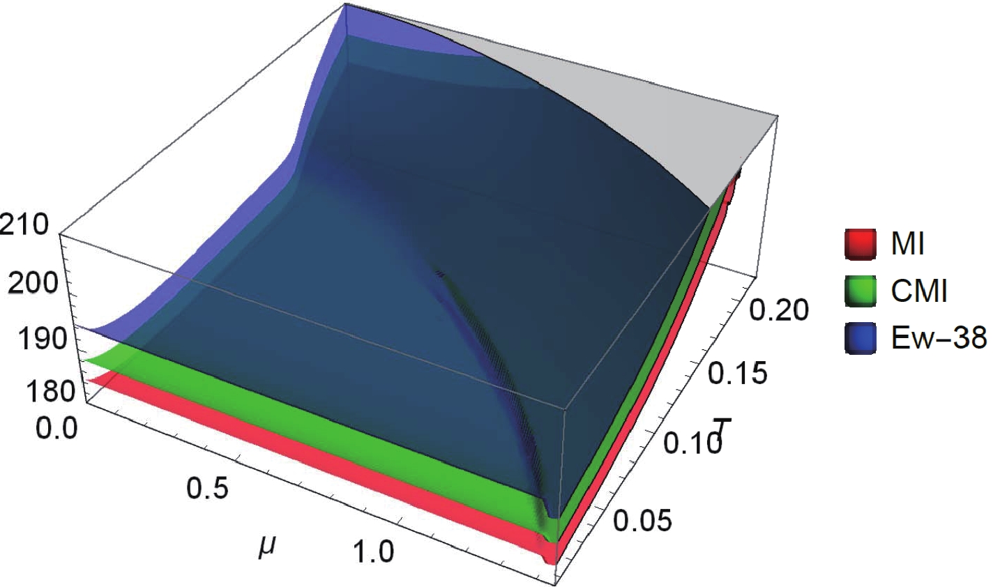

Figure 14.(color online) The mutual information (MI), conditional mutual information (CMI), and entanglement of purification(Ew) for case-3 ofAandBinTable 1.

The first " $ \geqslant $ " suggests that the maximal number of allowed bit threads that connectAandBis not equal to $ MI(A,B) $ or $ CMI(A,B|C) $ .

In this work, we investigated the holographic entanglement entropy of a holographic QCD model with a critical endpoint. We considered the behavior of entanglement entropy for a strip shaped region and a spherical shaped region on the phase diagram. It was determined that the behavior of holographic entanglement entropy on the phase diagram is independent of the shape of regionAexcept for the exact value, although the minimal area equations for differentAvalues are different. We also demonstrated how other entanglement quantities include mutual information, conditional mutual information, and the entanglement of purification behavior on the phase diagram. It was determined that the three entanglement quantities have very similar behavior: their values do not change significantly in the hadronic matter phase but increases rapidly with the increase inTand $ \mu $ in the QGP phase. Near the phase boundary, these three entanglement quantities change smoothly in the crossover region and continuously but not smoothly at CEP; they exhibit discontinuous behavior in the first phase transition region. Finally, we find an inequality for $ Ep(A,B) $ , $ I(A,B|C) $ and $ I(A,B) $

at anyTand $ \mu $ . This inequality suggests that the monogamy of $ I(A,B,C) $ is still satisfied, and $ Ep(A,B) $ is not the holographic duality of mutual information or conditional mutual information.

However, it should be noted that the black hole entropies for different holographic QCD models have a similar behavior. Even for $ \mu = 0 $ , the behavior of the holographic entanglement entropy does depend on the details of the hQCD models. For different hQCD models, the behavior of the holographic entanglement entropy on the (T, $ \mu $ ) phase diagram could be completely different. This indicates that the geometries of the bulk spacetime are completely different. In principle, the behavior of entanglement entropy between different subsystems of QCD matter should be unique. Therefore, the model dependence of holographic entanglement entropy indicates that bulk geometry must be addressed. One approach is to utilize machine learning [35,36]. An alternative method is to build a fully dynamic holographic QCD model. We are currently working on the latter.

We would like to thank Peng Liu for very helpful discussions.