


 Abstract
 HTML
HTML Reference
 Related
 PDF
PDF


-
As is well known, Einstein’s general relativity theory is non-renormalizable [1]. One of the most popular methods is to append all possible quadratic curvature invariants to the usual Einstein-Hilbert action [2], despite the existence of ghost-like modes in this theory. These terms constitute the so-called Einstein-Weyl (EW) gravity [3–5], which includes the most general Einstein-Hilbert action with quadratic curvature invariants. Subsequently, the non-Schwarzschild black hole (NSBH) solutions were recovered in four dimensional spacetime [3,4], where they also satisfy the condition of the Ricci scalar (
$ R = 0 $ ). Since the Ricci scalarRdoes not vanish in higher dimensional$ (n>4) $ spacetime, Lü et al. found only the perturbed numerical solutions in the EW gravity [6]. Employing the continued fraction method, Kokkotas et al. constructed a numerical black hole solution in an analytical form [7], and its Hawking radiation was discussed in Ref. [8]. Furthermore, some new solutions were derived in anti-de Sitter (AdS) spacetime [9,10].Recently, charged black holes were derived in Refs. [11-13] by applying the four dimensional EW theory coupled with an electromagnetic field. According to the ‘seed’ solution, these solutions can be divided into two groups in the Einstein-Maxwell-Weyl (EMW) theory. GroupIsolutions correspond to the charged extension of the higher derivative curvature for a Schwarzschild black hole. In GroupII, the solutions are constructed from the charged generalization of the NSBH solution. The thermodynamic properties of these charged black holes were investigated in Ref. [13].
The quasinormal modes (QNMs) of a black hole have been a hot research topic for decades. The concept of QNMs was introduced in 1957 by the work of Regge and Wheeler, who investigated the stability of black holes under small perturbations [14]. The study of QNMs is beneficial to the understanding of the structure of black hole spacetimes and could play an important role in the detection of gravitational waves and some fundamental symmetries for the gauge/gravity duality [15,16]. To date, QNMs have been calculated either by Einstein’s general relativity theory coupled with Maxwell theory [17-19] or nonlinear electrodynamics [20–24], or by modified gravities [25–28]. The analysis of QNMs of the non-Schwarzschild black holes was performed in the EW gravity [29,30], where the linear relation between QNM frequencies and the parameter
$ p = \frac{r_0}{\sqrt{2\alpha}} $ was recovered. Inspired by these results, we evaluate the effect of the chargeQon the QNMs and the stability of charged black holes in the Einstein-Maxwell-Weyl gravity. We will calculate the QNMs by considering test massless and massive scalar field perturbations on the charged black holes, respectively.This paper is constructed as follows. We first review charged black hole solutions with an increase of chargeQin the EMW gravity in Section 2. Then, we provide a detailed discussion of QNM frequencies under test scalar field perturbations, including massless and massive scalar fields in Section 3. Finally, we provide concluding remarks in the fourth section.
-
The action of the Einstein-Weyl gravity, combined with the electromagnetic field, is given by [12,13]
$ {\cal I} = \frac{1}{16\pi G}\int {\rm d}^{4}x \sqrt{-g}\left[R-\alpha C_{\mu\nu\rho\sigma}C^{\mu\nu\rho\sigma} -\kappa F_{\mu\nu}F^{\mu\nu}\right] , $

(1) where
$ F_{\mu\nu} = \nabla_{\mu}A_{\nu}-\nabla_{\nu}A_{\mu} $ is the electromagnetic tensor. Here,$ C_{\mu\nu\rho\sigma} $ is the Weyl tensor and the trace-free part of the Riemann tensor with the form [31,32]$ C_{\mu\nu\rho\sigma} = R_{\mu\nu\rho\sigma}-\left(g_{\mu[\rho}R_{\sigma]\nu}-g_{\nu[\rho}R_{\sigma]\mu}\right) +\frac{1}{3}R g_{\mu[\rho}R_{\sigma]\nu}, $

where the part within brackets surrounding the indices refers to the anti-symmetric part. To date, various attempts have been made to formulate the Weyl curvature hypothesis in a rigorous way. The simplest choice of a scalar constructed from the Weyl tensor is
$ C_{\mu\nu\rho\sigma}C^{\mu\nu\rho\sigma} $ from Eq. (1).The equations of motion are obtained as [12,13]
$\begin{split} {R_{\mu \nu }} - \frac{1}{2}{g_{\mu \nu }}R - 4\alpha {B_{\mu \nu }} - 2\kappa {T_{\mu \nu }} = 0,\quad {\nabla _\mu }{F^{\mu \nu }} =0, \end{split}$

(2) where
$ B_{\mu\nu} $ is the trace-free Bach tensor, and$ T_{\mu\nu} $ is energy-momentum tensor of the Maxwell field$\begin{split} {B_{\mu \nu }} =& \left( {{\nabla ^\rho }{\nabla ^\sigma } + \frac{1}{2}{R^{\rho \sigma }}} \right){C_{\mu \nu \rho \sigma }},\\ {T_{\mu \nu }} =& {F_{\alpha \mu }}F_{\;\nu }^\alpha - \frac{1}{4}{g_{\mu \nu }}{F_{\alpha \beta }}{F^{\alpha \beta }}. \end{split}$

(3) We choose the metric ansatz
$ \begin{split} {\rm d}s^2 = -N(r){\rm e}^{-2\delta(r)}{\rm d}t^2+\frac{1}{N(r)}{\rm d}r^2+r^2\left({\rm d}\theta^2+\sin^2\theta {\rm d}\varphi^2\right) \end{split}$

(4) with a metric function
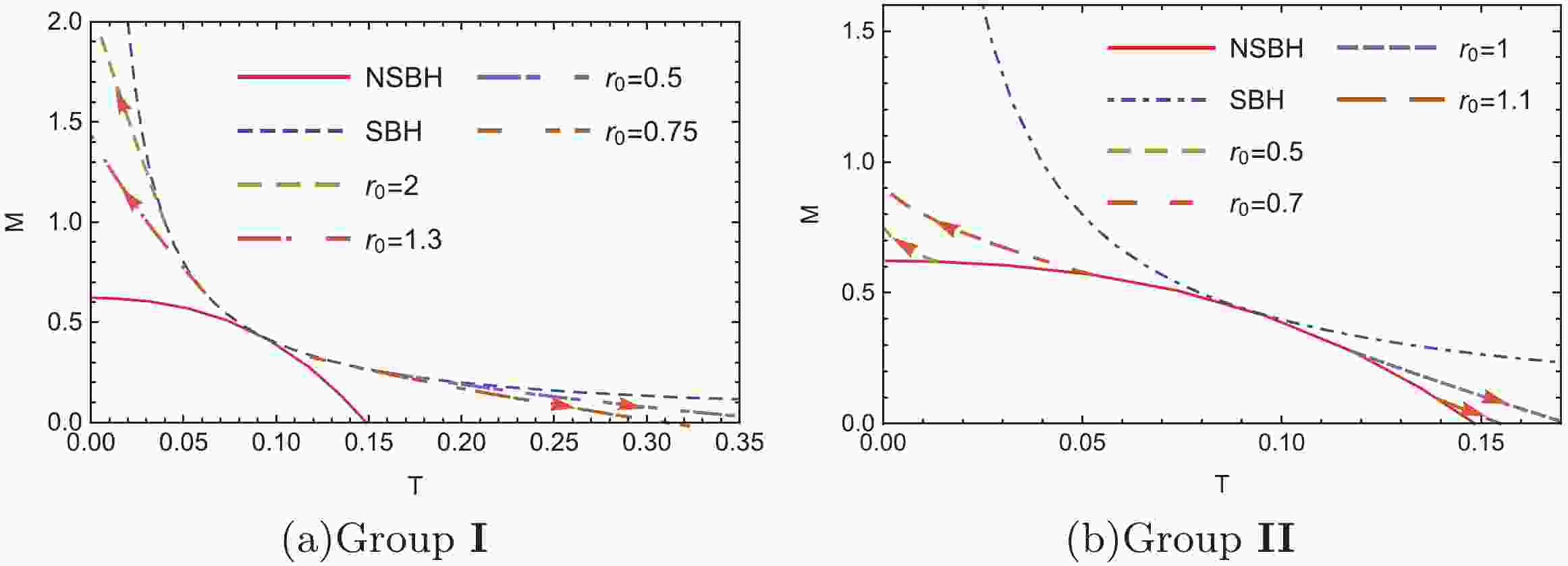
$ N(r) $ equal to$ 1-2m(r)/r $ . We constructed numerical charged black hole solutions with$ \alpha = \frac{1}{2} $ and$ \kappa = 1 $ [13], according to two neutral scenarios: the Schwarzschild (SBH) and non-Schwarzschild black hole (NSBH) within the bound of$ 0.363 in the EW theory.Fig. 1presents the relation between the massMand Hawking temperatureTfor SBH and NSBH scenarios, where both neutral solutions coalesce at$ T\approx0.091 (r_0\approx0.876) $ . Taking GroupI(Fig. 1(a)) as an example, charged black holes were constructed from the Schwarzschild black hole$ (Q = 0) $ by increasing the chargeQwhile maintaining the same horizon radius$ r_0 $ . In particular, new charged black holes on both sides of the coalescent point exhibit different properties: as the chargeQincreases, their mass becomes larger (smaller) depending on the temperature decrease (increase) on the left (right) hand side. A similar phenomenon is observed in GroupII, as shown inFig. 1(b).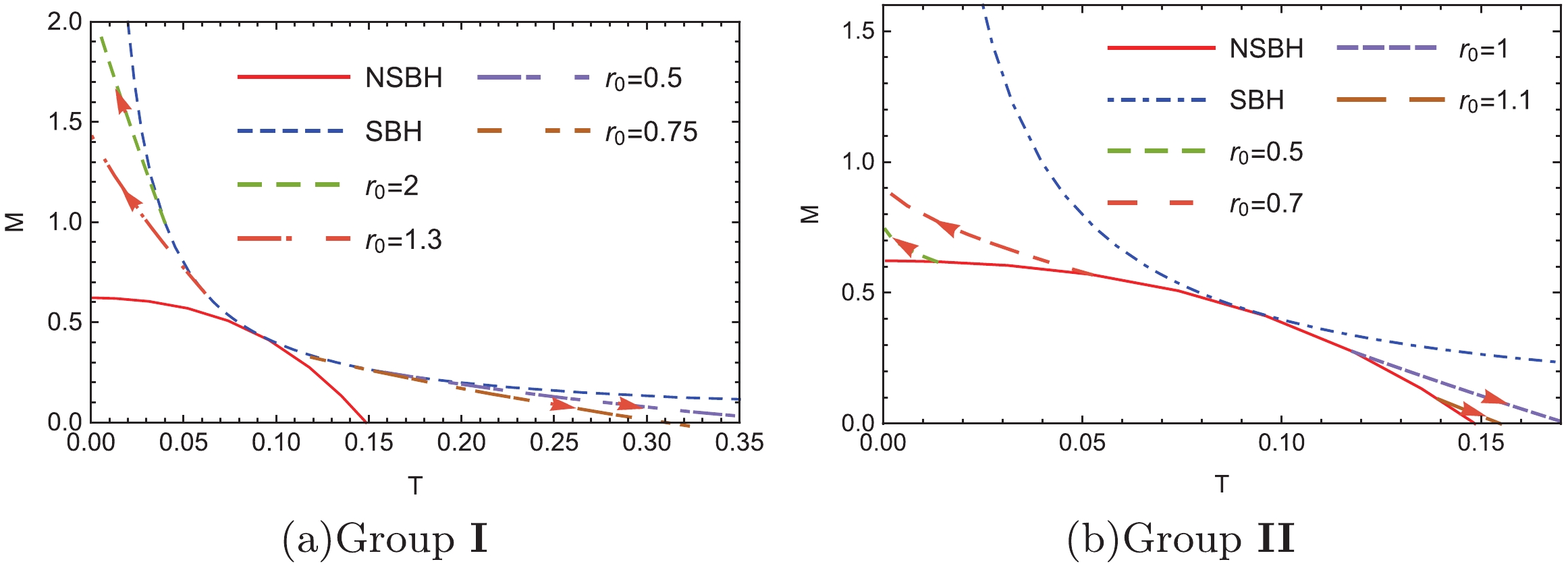
Figure 1.(color online) MassMversus temperatureTfor Schwarzschild (SBH), non-Schwarzschild (NSBH), and charged black holes for Group I (1) and Group II (b). The arrow denotes the increase in chargeQ.
-
In this section, we consider the test massive scalar field
$ \psi $ propagating on charged black holes, which obeys the Klein-Gordon equation$ \left(\square-\mu^2\right)\psi = 0, $

(5) where
$ \mu $ is the mass of the scalar field, and$ \psi $ can be separated into spherical harmonics, temporal, and radial components$\psi (t,r,\theta ,\phi ) = \sum\limits_{lm} {\frac{1}{r}} {\Psi _l}(r){Y_{lm}}(\theta ,\phi ){{\rm e}^{ -{\rm i}\omega t}},$

(6) where
$ Y_{lm}(\theta,\phi) $ is a usual spherical harmonic, andlis the angular harmonic index.Substituting Eqs. (4) and (6) into Eq. (5), we obtain the radial perturbed Schrödinger equation
$ \left(\partial^2_{r_*}+\omega^2-V_l(r)\right)\Psi_l(r) = 0, $

(7) where the effective potential is given as
$ V_l = \frac{l(l+1)N {\rm e}^{-2\delta}}{r^2}+\frac{N{\rm e}^{-2\delta}\left(N'-N\delta'\right)}{r} +\mu^2 N {\rm e}^{-2\delta} $

(8) and the tortoise coordinate
$ r_* $ is adopted as$ \frac{{\rm d}r_*}{{\rm d}r} = \frac{1}{N{\rm e}^{-\delta}}. $

(9) -
We consider the massless scalar field perturbation
$ (\mu = 0) $ in these charged black holes for GroupsIandII. First, we choose appropriate boundary conditions. The respective boundary conditions at the black hole horizon and spatial infinity are${\Psi _l}(r) \sim \left\{ {\begin{array}{*{20}{l}} {{{\rm e}^{ -{\rm i}\omega {r_*}}} \sim {{(r - {r_0})}^{ - \frac{{{\rm i}\omega }}{{4\pi T}}}}}&{r \to {r_0}({r_*} \to - \infty )}\\ {{{\rm e}^{{\rm i}\omega {r_*}}} \sim {{\rm e}^{ - {\rm i}\omega r}}{r^{2M{\rm i}\omega }}}&{r \to \infty ({r_*} \to \infty ),} \end{array}} \right.$

(10) To derive these QN modes
$ \omega $ , we employ the shooting method [33-35]. With the initial condition given by Eq. (10) at the event horizon$ r_0 $ , we solve the perturbed Eq. (7) numerically for each$ \omega $ using theWolfram Mathematica® built-in function NDSolve for$ r_0\leq r\leq r_f $ , where$ r_f\gg r_0 $ . This solution must also satisfy the boundary condition in Eq. (10) at spatial infinity, if$ \omega $ is the quasinormal frequency.In theTables 1–4, we present QNM frequencies (real and imaginary parts) for these charged black holes in GroupsIandII. The QNM frequencies (for
$ l = 0 $ and 1) of these neutral black holes (SBH and NSBH) are displayed in the first row ofTables 1–4. In the case of$ Q\rightarrow0 $ , the action presented in Eq. (1) becomes neutral [3,4], recovering the Schwarzschild and non-Schwarzschild solutions in four dimensional spacetime. The fundamental QNM frequencies under a massless scalar field perturbation on the SBH background are given in Refs. [36,37]. QNM frequencies (for$ l = 0 $ and 1) of the NSBH with a horizon radius$ r_0>0.876 $ are provided in Refs. [29,30]. However, for the NSBH with$ r_0<0.876 $ , there is a discrepancy between QNM frequencies and data obtained from the relation expression$ p\sim\omega $ in Ref. [30]. This is probably because this expression, derived in the bound$ 0.876 , is not valid in the region of$ 0.363 for the NSBH in the EW gravity.$r_0=0.5$ 

$r_0=0.75$ 

Q $\omega(l=0)$ 

$\omega(l=1)$ 

$\omega(l=0)$ 

$\omega(l=1)$ 

0 0.4420-0.4196i 1.1716-0.3908i 0.2947-0.2797i 0.7810-0.2605i 0.02 0.445730-0.419802i 1.17219-0.39126i 0.29504-0.284839i 0.781750-0.262508i 0.06 0.447649-0.423259i 1.17636-0.394006i 0.300096-0.291943i 0.768417-0.266851i 0.1 0.451833-0.431002i 1.18541-0.399437i 0.305035-0.307715i 0.795061-0.269681i 0.14 0.458975-0.443435i 1.19959-0.408586i 0.310574-0.309508i 0.806376-0.275657i 0.18 0.465102-0.456727i 1.21463-0.420002i 0.315876-0.317400i 0.820854-0.281226i 0.22 0.467173-0.461698i 1.23312-0.434605i 0.318256-0.328687i 0.825449-0.304661i 0.26 0.481790-0.486744i 1.25409-0.445270i 0.321404-0.342171i 0.830678-0.326003i 0.30 0.512190-0.519842i 1.27810-0.477936i 0.324608-0.355701i 0.834912-0.334916i 0.33 0.522566-0.532159i 1.29662-0.490691i 0.330838-0.369421i 0.838476-0.351239i Table 1.QNM frequencies of black holes within region ofr0< 0.876 in GroupI.
$r_0=1.3$ 

$r_0=2$ 

Q $\omega(l=0)$ 

$\omega(l=1)$ 

$\omega(l=0)$ 

$\omega(l=1)$ 

0 0.1700-0.1614i 0.4506-0.1503i 0.1105-0.1049i 0.2929-0.0977i 0.02 0.169935-0.160131i 0.449981-0.149923i 0.110434-0.104754i 0.292409-0.0975053i 0.06 0.169604-0.158960i 0.449018-0.149611i 0.110072-0.104079i 0.290913-0.0960668i 0.1 0.169109-0.157354i 0.448207-0.148787i 0.108803-0.101841i 0.287647-0.0937670i 0.14 0.168720-0.155810i 0.447165-0.147679i 0.106439-0.098191i 0.283246-0.0906137i 0.18 0.168023-0.153998i 0.443449-0.145653i 0.103804-0.0933381i 0.278075-0.0869171i 0.22 0.166891-0.151193i 0.441312-0.143235i 0.101889-0.0875931i 0.272255-0.0830565i 0.26 0.166014-0.148333i 0.437092-0.140916i 0.100331-0.0820946i 0.266262-0.0790222i 0.30 0.165430-0.144852i 0.432538-0.137778i 0.098978-0.0771625i 0.259892-0.0749341i 0.33 0.164395-0.143688i 0.429952-0.135908i 0.098060-0.0736714i 0.254996-0.0719146i Table 2.QNM frequencies of black holes within region ofr0> 0.876 in GroupI.
$r_0=0.5$ 

$r_0=0.7$ 

Q $\omega(l=0)$ 

$\omega(l=1)$ 

$\omega(l=0)$ 

$\omega(l=1)$ 

0 0.1920-0.05801i 0.5650-0.1168i 0.2484-0.1550i 0.5574-0.4347i 0.02 0.191974-0.0578165i 0.563943-0.115416i 0.247626-0.15488i 0.556522-0.433647i 0.06 0.191900-0.0575649i 0.561869-0.114350i 0.245508-0.153018i 0.551806-0.407181i 0.1 0.191801-0.0572173i 0.556545-0.112453i 0.242262-0.150052i 0.550735-0.410594i 0.12 0.191707-0.0569421i 0.553771-0.111982i 0.240109-0.148196i 0.548074-0.403119i 0.155 0.191457-0.0563484i 0.547261-0.109390i 0.235633-0.144682i 0.542076-0.386617i 0.185 0.191279-0.0559977i 0.543921-0.104531i 0.231188-0.141623i 0.536208-0.369774i 0.215 0.190982-0.0555578i 0.534453-0.100874i 0.226304-0.138735i 0.530038-0.353073i 0.25 0.188420-0.0548792i 0.521852-0.094748i 0.220221-0.135954i 0.518341-0.344284i 0.29 0.185355-0.0536175i 0.508852-0.087635i 0.213025-0.133582i 0.508015-0.333045i Table 3.QNM frequencies of black holes within region ofr0< 0.876 in GroupII.
$r_0=1$ 

$r_0=1.1$ 

Q $\omega(l=0)$ 

$\omega(l=1)$ 

$\omega(l=0)$ 

$\omega(l=1)$ 

0 0.2490-0.3900i 0.6920-0.2920i 0.2967-0.4970i 0.7764-0.3774i 0.02 0.248326-0.390859i 0.697313-0.292519i 0.298359-0.497294i 0.78196-0.3774330i 0.055 0.249730-0.398086i 0.699694-0.294816i 0.300096-0.497879i 0.786675-0.377930i 0.09 0.251139-0.403061i 0.706433-0.300164i 0.303839-0.507651i 0.795747-0.387478i 0.125 0.258110-0.418834i 0.713570-0.308565i 0.313144-0.495390i 0.795217-0.390079i 0.16 0.257806-0.426266i 0.722897-0.314524i 0.315173-0.529731i 0.816878-0.410238i 0.195 0.262761-0.434169i 0.731343-0.322654i 0.322461-0.538773i 0.827657-0.422568i 0.23 0.266851-0.445229i 0.740003-0.332937i 0.328884-0.559389i 0.842650-0.437051i 0.28 0.279679-0.465540i 0.749440-0.341363i 0.341379-0.571647i 0.860521-0.459423i Table 4.QNM frequencies of black holes within region ofr0> 0.876 in GroupII.
For charged black holes, the imaginary parts are always negative, indicating that these modes always decay and are therefore stable. Moreover, for the charged black holes with
$ r_0 = 0.5 $ and 0.75 in GroupI, the absolute values of the imaginary part$ (\left|\omega_i\right|) $ and real part$ (\omega_r) $ of QNM frequencies$ (l = 0,1) $ both increase with increasing ofQ(seeTable 1andFig. 2(a)). In contrast, the corresponding values of$ \left|\omega_i\right| $ and$ \omega_r $ of QNM frequencies for charged black holes with$ r_0 = 1.3 $ and 2 in GroupIboth decrease with increasing ofQ(seeTable 2andFig. 2(b)). Similarly, QNM frequencies of these charged black holes in GroupII,located each side of the coalescent point$ T\approx0.091(r_0\approx0.876) $ , exhibit different trends from the ones given inTables 3,4andFig. 3. This is because the massMand temperatureTof these charged black holes affect the boundary conditions of the test scalar field$ \Psi_l(r) $ given in Eq. (10). However, based on the free energies (Fig. 7 in Ref. [13]) and QNM frequencies of these charged and neutral black holes [Figs. 2and3], the correlation between thermodynamic phase transitions and dynamical stabilities fails.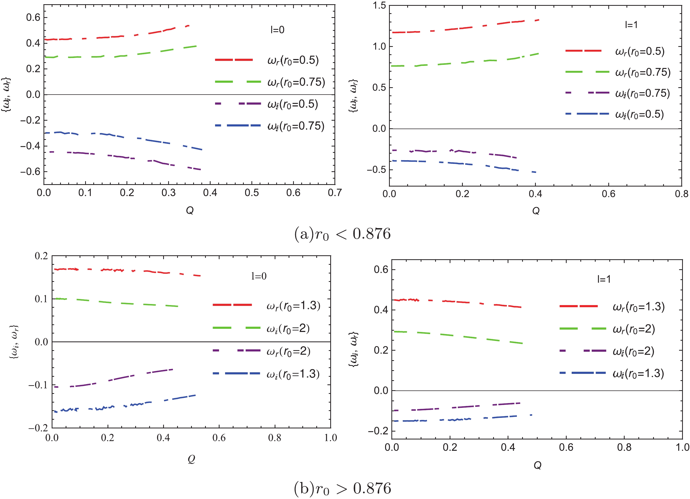
Figure 2.(color online) Dependence of fundamental QNM frequencies of charged black hole on chargeQwith fixed horizon radius in GroupI.
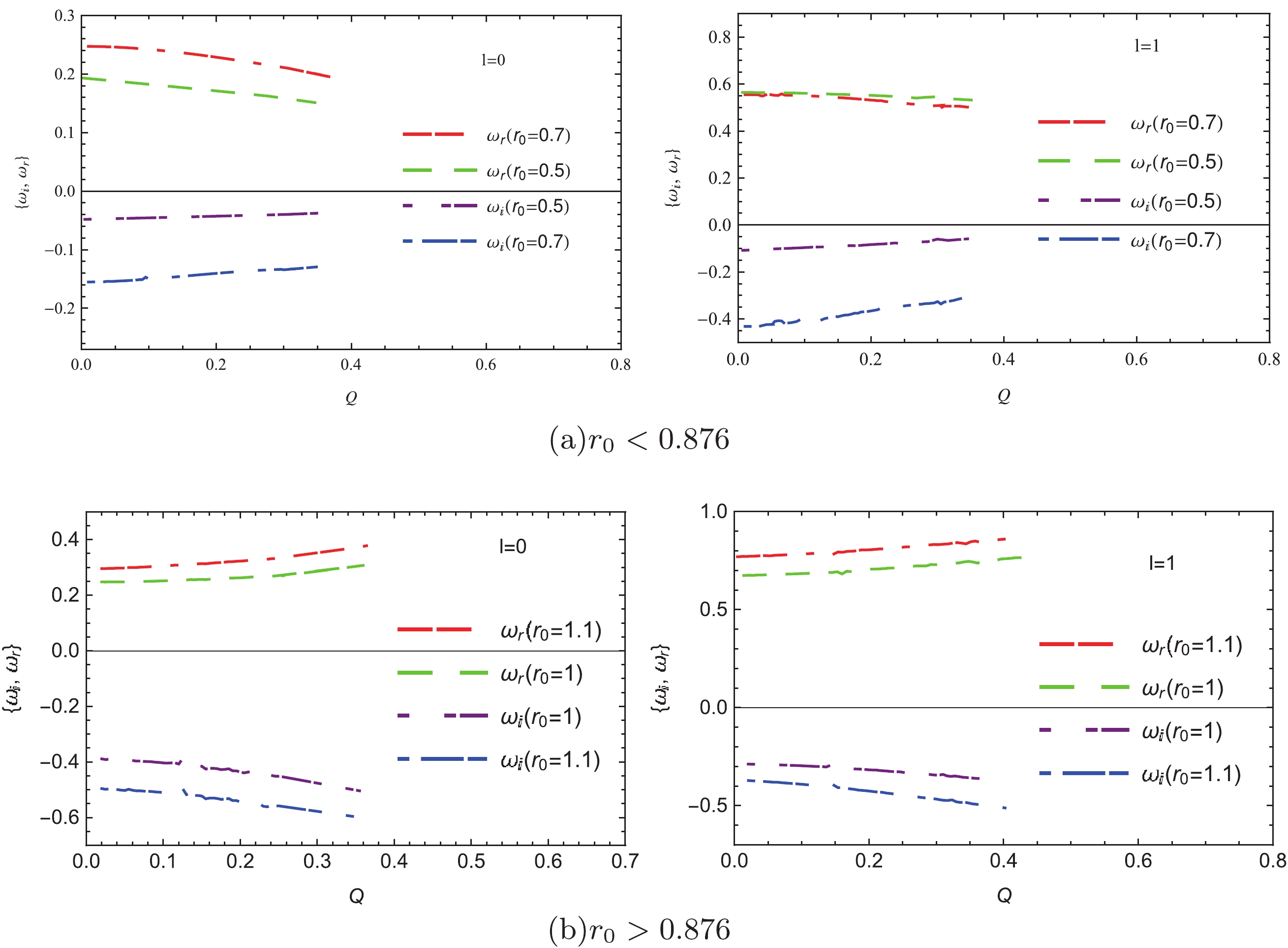
Figure 3.(color online) Dependence of fundamental QNM frequencies of charged black hole on chargeQwith fixed horizon radius in GroupII.
Notably, the study of Ref. [30] asserted that QNM frequencies
$ \omega $ are linearly dependent on$ p = \frac{r_0}{\sqrt{2\alpha}} $ for NSBH in the EW gravity. Following a similar path, we assume$ \alpha = 1/2 $ and a fixed chargeQ, and subsequently consider QNMs of the new charged black holes with a different horizon radius$ r_0 $ (here, we do not show new numerical solutions) for various multipole numbersl,assuming$ p = \frac{r_0}{\sqrt{2\alpha}} = r_0 $ . According to QNM frequencies of charged black holes with$ r_0 = p = 0.5 $ in GroupIand$ r_0 = p = 0.7 $ in GroupII, these new QNM frequencies are expressed as a function ofpinTable 5andFigs. 4and5. In comparison with QNMs of charged black holes with$ p = r_0 = 0.5 $ , the new charged black holes with different values of$ p = r_0>0.5 $ exhibit lower real frequencies and a lower damping rate. Moreover, the tendency of the imaginary part of QNM frequencies for$ l = 1 $ changes, as shown inFig. 5(b). Finally, we do not observe the strict linear relation between$ \omega $ andp, as the chargeQcauses a nonlinear effect on the frequency for these charged black holes in the EMW gravity.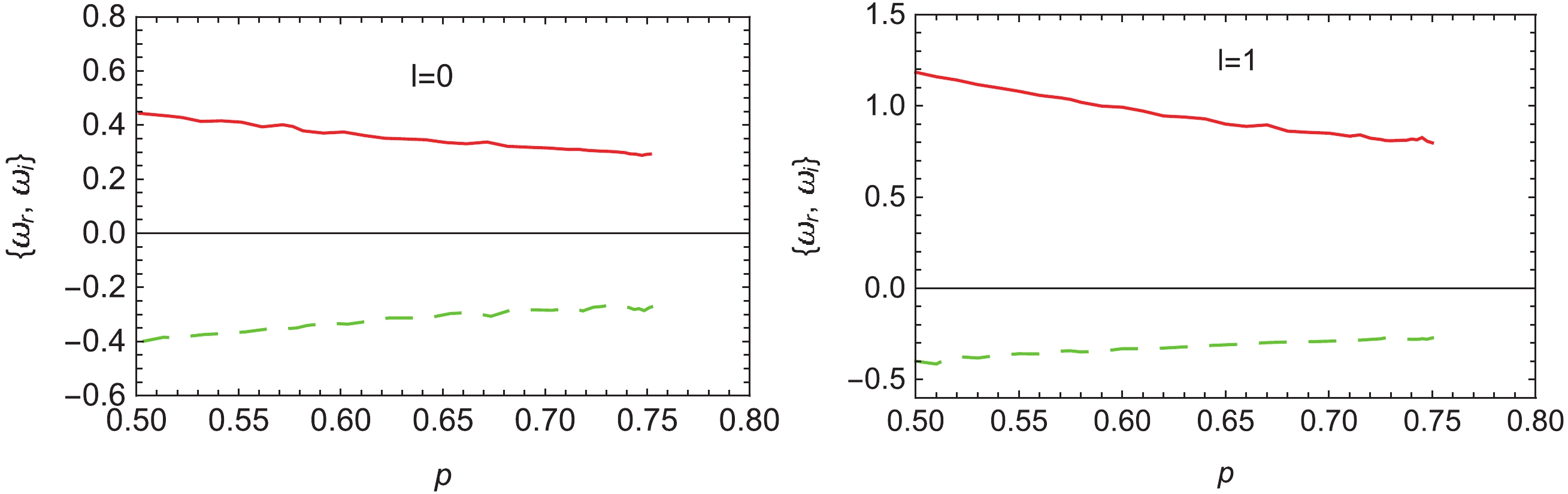
Figure 4.(color online) Dependence of QNM frequencies of charged black hole on parameterpwith
$Q=0.1$ starting from$Q=0.1$ and$p=r_0=0.5$ in GroupI. Solid and dashed lines denote the real and imaginary parts of QNM frequencies, respectively.GroupI GroupII p $\omega(l=0)$ 

$\omega(l=1)$ 

p $\omega(l=0)$ 

$\omega(l=1)$ 

0.5 0.451303-0.428182i 1.185030-0.399112i 0.7 0.242462-0.150258i 0.551352-0.409716i 0.54 0.423578-0.399711i 1.099260-0.366381i 0.685 0.242485-0.150641i 0.560200-0.387280i 0.58 0.386467-0.369919i 1.019980-0.348577i 0.665 0.242862-0.151787i 0.568930-0.372865i 0.63 0.356692-0.342205i 0.939253-0.320923i 0.65 0.243282-0.153298i 0.574191-0.367385i 0.68 0.329482-0.312415i 0.862011-0.294039i 0.64 0.243481-0.155328i 0.583836-0.360624i 0.72 0.313943-0.302641i 0.823348-0.279923i 0.62 0.244227-0.162025i 0.601820-0.359452i 0.75 0.300831-0.297926i 0.797623-0.271460i 0.6 0.246600-0.169481i 0.60298-0.346543i Table 5.Dependence of QNM frequencies of charged black hole on parameterpwith fixed
$Q=0.1$ in GroupsIandII.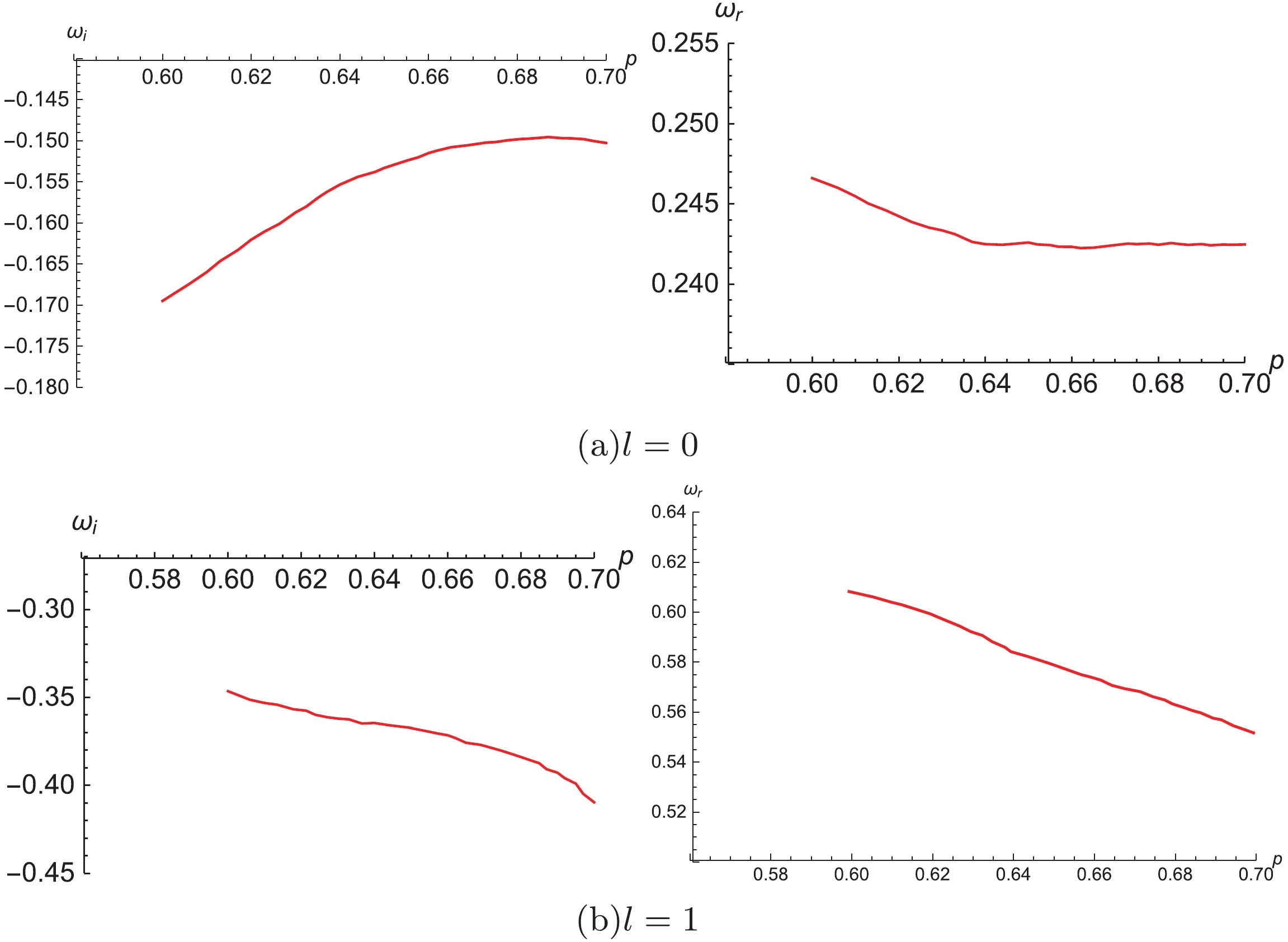
Figure 5.(color online) Dependence of QNM frequencies of charged black hole on parameterpwith
$Q=0.1$ starting from$Q=0.1$ and$p=r_0=0.7$ in GroupII. -
We consider how the behavior of QNMs changes depending on the massive scalar field
$ \mu\neq0 $ . Under the massive scalar field perturbation, the boundary conditions are different from those in the massless case. From the radial perturbed Schrödinger Eq. (7), the respective ingoing boundary conditions at the black hole event horizon and outgoing boundary conditions at spatial infinity are obtained as${\Psi _l}(r) \sim \left\{ {\begin{array}{*{20}{l}} {{{\rm e}^{ -{\rm i}\omega {r_*}}} \sim {{(r - {r_0})}^{ - \frac{{{\rm i}\omega }}{{4\pi T}}}},}&{r \to {r_0}}\\ {{{\rm e}^{{\rm i}{{({\mu ^2} - {\omega ^2})}^{1/2}}{r_*}}} \sim {{rm e}^{ - {{({\mu ^2} - {\omega ^2})}^{1/2}}r}}{r^{ - 2M{{({\mu ^2} - {\omega ^2})}^{1/2}}}}}&{r \to \infty } \end{array}} \right.$

(11) We take as an example the charged black holes with
$ r_0 = 0.5 $ and$ Q = 0.1 $ in GroupI. The QNM frequencies as a function of mass$ \mu $ are shown inFig. 6[38]. For the angular parameter$ l = 0 $ , the real part of the QNM frequencies becomes larger, while the imaginary part decreases with increasing mass$ \mu $ . This indicates that massive modes are scattered more slowly than massless modes. Moreover, these oscillations could become undamped, i.e.,$ \omega_i = 0 $ , under certain conditions, causing the appearance of so-called quasiresonances. This phenomenon emerged for the massive scalar field perturbation in the NSBH background in EW gravity [30] and the charged field perturbation in the RN black hole [39,40,41]. Nevertheless, these quasiresonances disappear for$ l = 1 $ in the EMW gravity.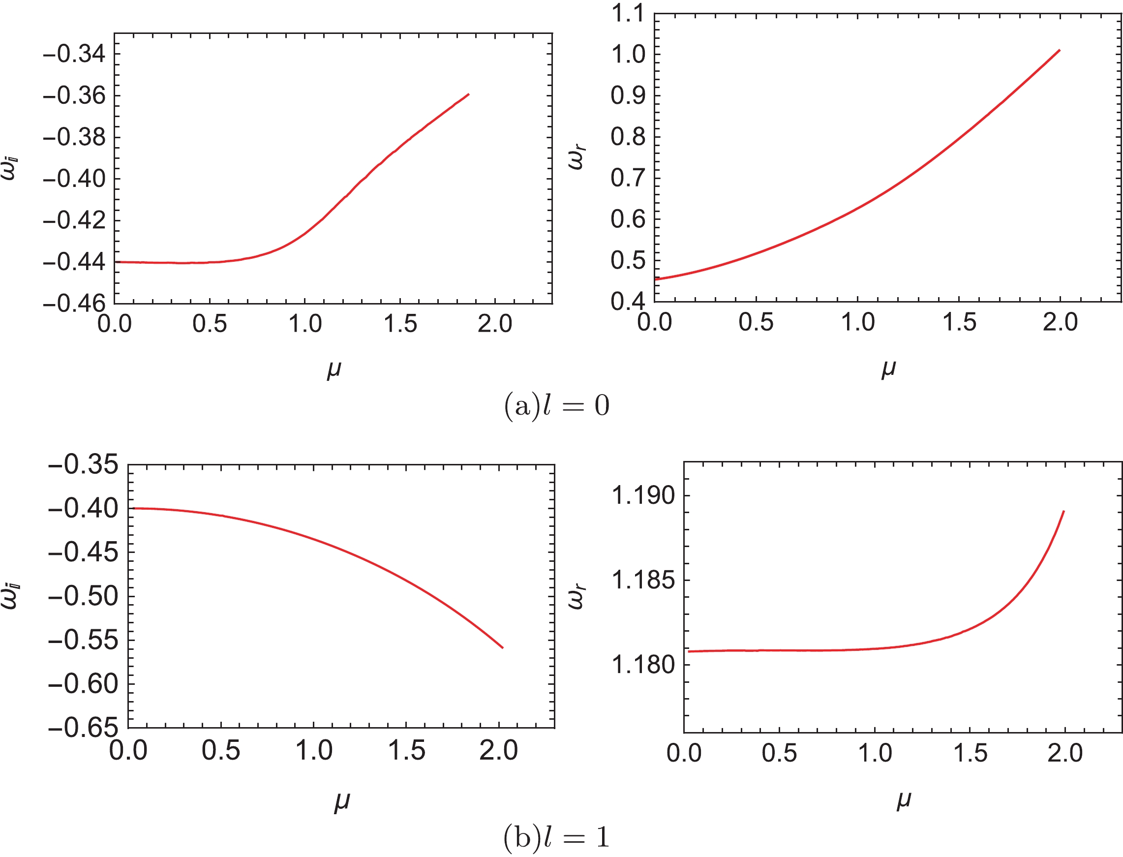
Figure 6.(color online) Dependence of QNM frequencies of charged black hole on mass \mu with
$ r_0 = 0.5 $ and$ Q = 0.1 $ in GroupIon the mass . -
Applying the Einstein-Maxwell-Weyl theory, we investigated QNMs and the stability of charged black holes under the test scalar field perturbation. With an increase in the chargeQ, QNM frequencies are depicted by larger (smaller) real oscillations and higher (lower) damping rates, than those for the neutral branches at the same side of the coalescent point
$ T\approx0.091(r_0\approx0.876) $ , in both GroupsIandII. Moreover, these phenomena are reflected by the behaviors of the thermodynamic quantitiesMandT. Furthermore, the linear dependence of the QNM frequency on the parameterpfor NSBH in the EW gravity does not manifest for the new charged black holes in the EMW gravity, as the chargeQcauses a nonlinear effect on QNM frequencies. Furthermore, we discussed the case of a massive scalar field perturbation, where undamped oscillations occur for sufficiently large masses.Recently, (anti-) de Sitter charged black hole solutions in the EMW gravity were presented [11]. Because of the dual conformal field theory, QNM frequencies of AdS black holes have a direct interpretation [42,43]. Therefore, it would be interesting to consider QNMs and the stability of charged AdS black holes in the EMW gravity.
Quasinormal modes of charged black holes in Einstein-Maxwell-Weyl gravity
- Received Date:2019-09-18
- Accepted Date:2019-11-19
- Available Online:2020-05-01
Abstract:We study quasinormal modes (QNMs) of charged black holes in the Einstein-Maxwell-Weyl (EMW) gravity by adopting the test scalar field perturbation. We find that the imaginary part of QNM frequencies is consistently negative for different angular parametersl, indicating that these modes always decay and are therefore stable. We do not observe a linear relationship between the QNM frequencyωand parameterpfor these black holes, as their chargeQcauses a nonlinear effect. We evaluate the massive scalar field perturbation in charged black holes and find that random long lived modes (i.e., quasiresonances) could exist in this spectrum.


 DownLoad: